Sea ice plotting examples
This script shows how to load and plot sea ice concentration from sea ice models (CICE5, and SIS2) output, while also indicating how to get around some of the pitfalls and foibles in CICE temporal and spatial gridding.
Requirements: The conda/analysis3 module from /g/data/hh5/public/modules.
[1]:
#Choose which model we are working with
MODEL='cice5'
# MODEL='sis2'
Firstly, load modules:
[2]:
import cosima_cookbook as cc
from dask.distributed import Client
from datetime import timedelta
import cf_xarray as cfxr

import matplotlib.pyplot as plt
import cartopy.crs as ccrs
import cartopy.feature as cfeature
import numpy as np
import matplotlib.path as mpath
import cmocean.cm as cmo
[3]:
client = Client()
client
[3]:
Client
Client-5fbc968e-6b60-11ee-80a3-00000751fe80
| Connection method: Cluster object | Cluster type: distributed.LocalCluster |
| Dashboard: /proxy/8787/status |
Cluster Info
LocalCluster
50bc1efc
| Dashboard: /proxy/8787/status | Workers: 7 |
| Total threads: 28 | Total memory: 112.00 GiB |
| Status: running | Using processes: True |
Scheduler Info
Scheduler
Scheduler-67f3cd42-6c5d-4551-9821-1daab7b671a7
| Comm: tcp://127.0.0.1:34609 | Workers: 7 |
| Dashboard: /proxy/8787/status | Total threads: 28 |
| Started: Just now | Total memory: 112.00 GiB |
Workers
Worker: 0
| Comm: tcp://127.0.0.1:34497 | Total threads: 4 |
| Dashboard: /proxy/43673/status | Memory: 16.00 GiB |
| Nanny: tcp://127.0.0.1:36635 | |
| Local directory: /jobfs/98205487.gadi-pbs/dask-scratch-space/worker-6r3t08wh | |
Worker: 1
| Comm: tcp://127.0.0.1:46043 | Total threads: 4 |
| Dashboard: /proxy/33069/status | Memory: 16.00 GiB |
| Nanny: tcp://127.0.0.1:34243 | |
| Local directory: /jobfs/98205487.gadi-pbs/dask-scratch-space/worker-d42m636r | |
Worker: 2
| Comm: tcp://127.0.0.1:38617 | Total threads: 4 |
| Dashboard: /proxy/46515/status | Memory: 16.00 GiB |
| Nanny: tcp://127.0.0.1:44115 | |
| Local directory: /jobfs/98205487.gadi-pbs/dask-scratch-space/worker-qsg86muz | |
Worker: 3
| Comm: tcp://127.0.0.1:33653 | Total threads: 4 |
| Dashboard: /proxy/36275/status | Memory: 16.00 GiB |
| Nanny: tcp://127.0.0.1:42325 | |
| Local directory: /jobfs/98205487.gadi-pbs/dask-scratch-space/worker-bmavhh68 | |
Worker: 4
| Comm: tcp://127.0.0.1:35511 | Total threads: 4 |
| Dashboard: /proxy/36113/status | Memory: 16.00 GiB |
| Nanny: tcp://127.0.0.1:46195 | |
| Local directory: /jobfs/98205487.gadi-pbs/dask-scratch-space/worker-y16un6x3 | |
Worker: 5
| Comm: tcp://127.0.0.1:34521 | Total threads: 4 |
| Dashboard: /proxy/42057/status | Memory: 16.00 GiB |
| Nanny: tcp://127.0.0.1:37443 | |
| Local directory: /jobfs/98205487.gadi-pbs/dask-scratch-space/worker-shz_8g77 | |
Worker: 6
| Comm: tcp://127.0.0.1:34155 | Total threads: 4 |
| Dashboard: /proxy/35385/status | Memory: 16.00 GiB |
| Nanny: tcp://127.0.0.1:35911 | |
| Local directory: /jobfs/98205487.gadi-pbs/dask-scratch-space/worker-_5j2riy4 | |
Start a database session:
[4]:
session = cc.database.create_session()
The dictionary below specifies experiment, start and ending times for each model we can use (CICE5 with MOM5 or SIS2 with MOM6). This example will work with RYF forcing experiments and sea ice concentration variable, which is called aice_m in mom5 and siconc in mom6.
If you want a different experiment, or a different time period, change the necessary values. A tutorial on how to explore the database for available experiments is available here. Note that we are just loading the last 10 years here.
Note also the decode_coords=False flag. This gets around some messy issues with the way xarray decides to load CICE grids:
[5]:
sic_args = {
    "cice5": { #cice5 is part of ACCESS-OM2
        "expt": "01deg_jra55v13_ryf9091",
        "variable": "aice_m",
        "start_time": "1981-02-01",
        "end_time": "1991-01-01",
        "decode_coords": False
    },
    "sis2": { #sis2 is used for the testing MOM6
        "expt": "OM4_025.JRA_RYF",
        "variable": "siconc",
        "start_time": "1981-01-01",
        "end_time": "1990-12-31",
        "frequency": "1 monthly"
    },
    #In the future, we will add a CICE6 option (i.e. the future ACCESS-OM3)
}

area_variable = {
    "cice5": "area_t" ,
    "sis2": "areacello"
}

geo_variables = {
    "cice5":['geolon_t', 'geolat_t'] ,
    "sis2": ['geolon', 'geolat']
}
[6]:
sic = cc.querying.getvar(
    session=session,
    **sic_args[MODEL]
)
Another messy thing about CICE is that it thinks that monthly data for, say, January occurs at midnight on Jan 31 – while xarray interprets this as the first milllisecond of February.
To get around this, note that we loaded data from February above, and we now subtract 12 hours from the time dimension. This means that, at least data is sitting in the correct month, and really helps to compute monthly climatologies correctly.
[7]:
if MODEL =='cice5' :
    sic['time'] = sic.time.to_pandas() - timedelta(hours = 12)
[8]:
sic = sic.chunk([3, 'auto', 'auto'])
sic
[8]:
<xarray.DataArray 'aice_m' (time: 120, nj: 2700, ni: 3600)>
dask.array<rechunk-merge, shape=(120, 2700, 3600), dtype=float32, chunksize=(3, 2700, 3600), chunktype=numpy.ndarray>
Coordinates:
  * time     (time) object 1981-01-31 12:00:00 ... 1990-12-31 12:00:00
Dimensions without coordinates: nj, ni
Attributes: (12/13)
    units:          1
    long_name:      ice area  (aggregate)
    coordinates:    TLON TLAT time
    cell_measures:  area: tarea
    cell_methods:   time: mean
    time_rep:       averaged
    ...             ...
    contact:        Andy Hogg
    email:          andy.hogg@anu.edu.au
    created:        2020-06-11
    description:    0.1 degree ACCESS-OM2 global model configuration with JRA...
    notes:          Additional daily outputs saved from 1 Jan 1950 to 31 Dec ...
url: https://github.com/COSIMA/01deg_jra55_ryf/tree/01deg_jra5...Note that aice_m is the monthly average of fractional ice area in each grid cell aka the concentration. To find the actual area of the ice we need to know the area of each cell. Unfortunately, CICE doesn’t save this for us … but the ocean model does. So, let’s load area_t from the ocean model, and rename the coordinates in our ice variable to match the ocean model. Then we can multiply the ice concentration with the cell area to get a total ice area.
[9]:
area = cc.querying.getvar(sic_args[MODEL]['expt'], area_variable[MODEL], session, n = 1).load()

if MODEL=="sis2":
    area=area.rename({'xh': 'xT', 'yh': 'yT'})

area
[9]:
<xarray.DataArray 'area_t' (yt_ocean: 2700, xt_ocean: 3600)>
array([[nan, nan, nan, ..., nan, nan, nan],
       [nan, nan, nan, ..., nan, nan, nan],
       [nan, nan, nan, ..., nan, nan, nan],
       ...,
       [nan, nan, nan, ..., nan, nan, nan],
       [nan, nan, nan, ..., nan, nan, nan],
       [nan, nan, nan, ..., nan, nan, nan]], dtype=float32)
Coordinates:
  * xt_ocean  (xt_ocean) float64 -279.9 -279.8 -279.7 ... 79.75 79.85 79.95
  * yt_ocean  (yt_ocean) float64 -81.11 -81.07 -81.02 ... 89.89 89.94 89.98
    geolon_t  (yt_ocean, xt_ocean) float32 nan nan nan nan ... nan nan nan nan
    geolat_t  (yt_ocean, xt_ocean) float32 nan nan nan nan ... nan nan nan nan
Attributes:
    long_name:     tracer cell area
    units:         m^2
    valid_range:   [0.e+00 1.e+15]
    cell_methods:  time: point
    ncfiles:       ['/g/data/ik11/outputs/access-om2-01/01deg_jra55v13_ryf909...
    contact:       Andy Hogg
    email:         andy.hogg@anu.edu.au
    created:       2020-06-11
    description:   0.1 degree ACCESS-OM2 global model configuration with JRA5...
    notes:         Additional daily outputs saved from 1 Jan 1950 to 31 Dec 1...
url: https://github.com/COSIMA/01deg_jra55_ryf/tree/01deg_jra55...Our CICE data is missing x&y coordinate values, so we can also get them from area_t
So that our new coordinates are recognised as cf standard, we also need to copy the attributes. This notebook is designed to use cf-xarray. This means the rest of the notebook is Model Agnostic.
[10]:
if MODEL =='cice5' :
    sic.coords['ni'] = area['xt_ocean'].values
    sic.coords['nj'] = area['yt_ocean'].values

    sic.ni.attrs = area.xt_ocean.attrs
    sic.nj.attrs = area.yt_ocean.attrs

    sic = sic.rename(({'ni': 'xt_ocean', 'nj': 'yt_ocean'}))
[11]:
sic.cf
[11]:
Coordinates:
             CF Axes: * X: ['xt_ocean']
                      * Y: ['yt_ocean']
                        Z, T: n/a

      CF Coordinates: * longitude: ['xt_ocean']
                      * latitude: ['yt_ocean']
                        vertical, time: n/a

       Cell Measures:   area, volume: n/a

      Standard Names:   n/a

              Bounds:   n/a

       Grid Mappings:   n/a
Now that we have axes with cf compliant coordinates, we can select using latitude keywords.
Sea Ice Area
Let’s look at a timeseries of SH sea ice area. Area is defined (per convention) as the sum of sea ice concentration multiply by the area of each grid cell (and masked for sea ice concentration above 15%)
By convention, sea-ice area for a region or basin is the sum of the area’s where concentration is greater than 15%. We also need to drop geolon and geolat so we have unique longitude and latitude to reference
[12]:
sic = sic.where(sic >= 0.15)

si_area = sic * area

if MODEL=='cice5':
    si_area = si_area.drop({'geolon_t', 'geolat_t'})
[13]:
si_area.cf
[13]:
Coordinates:
             CF Axes: * X: ['xt_ocean']
                      * Y: ['yt_ocean']
                        Z, T: n/a

      CF Coordinates: * longitude: ['xt_ocean']
                      * latitude: ['yt_ocean']
                        vertical, time: n/a

       Cell Measures:   area, volume: n/a

      Standard Names:   n/a

              Bounds:   n/a

       Grid Mappings:   n/a
[14]:
SH_area = si_area.cf.sel(latitude=slice(-90, -45)).cf.sum(['latitude', 'longitude'])
NH_area = si_area.cf.sel(latitude=slice(45, 90)).cf.sum(['latitude', 'longitude'])
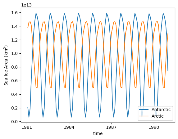
As we are using a repeat year forcing experiemnt, the sea ice cycle is very regular:
[15]:
SH_area.plot(label = 'Antarctic')
NH_area.plot(label = 'Arctic')

plt.legend(loc='lower right')
plt.ylabel('Sea Ice Area (km$^{2}$)');
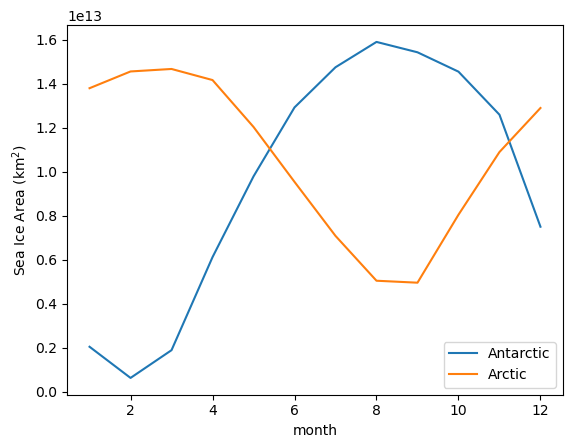
And the seasonal cycle of sea-ice area:
[16]:
SH_area.groupby('time.month').mean('time').plot(label='Antarctic')
NH_area.groupby('time.month').mean('time').plot(label='Arctic')

plt.legend()
plt.ylabel('Sea Ice Area (km$^{2}$)');
Making Maps
If we just plot a selected month now, you see that everything North of 65N is skewed.
[17]:
ax = plt.subplot(projection = ccrs.PlateCarree())

sic.sel(time='1985-08').plot(cmap = cmo.ice)
ax.coastlines();
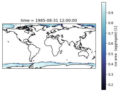
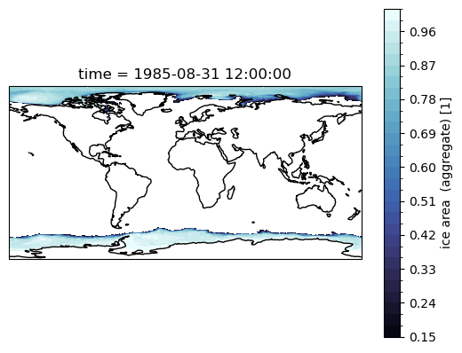
Most of our work is in the Southern Ocean, so maybe we don’t care. But if you are interested in the Arctic, then we need to account for the tri-polar ocean grid that out models use. The easiest way out of that is using contourf, and the passing the x and y coordinates.
See Making Maps with Cartopy tutorial for more help with plotting!
We need the geolon and geolat fields from the model for the actual (two-pole) coordinates, instead of the model (three-pole) coordinates.
[18]:
geolon = cc.querying.getvar(sic_args[MODEL]['expt'], geo_variables[MODEL][0], session, n = 1).load()
geolat = cc.querying.getvar(sic_args[MODEL]['expt'], geo_variables[MODEL][1], session, n = 1).load()

if MODEL=='sis2':
    geolon = geolon.rename({'lath': 'yT','lonh': 'xT'})
    geolat = geolat.rename({'lath': 'yT','lonh': 'xT'})
[19]:
sic=sic.assign_coords({
    'geolat': geolat,
    'geolon': geolon
})
Use contourf, and the geolon and geolat fields
[20]:
ax = plt.subplot(projection=ccrs.PlateCarree())

sic.sel(time='1985-08').squeeze('time').plot.contourf(
    transform = ccrs.PlateCarree(),
    x = 'geolon',
    y = 'geolat',
    levels = 33,
    cmap = cmo.ice
)

ax.coastlines();
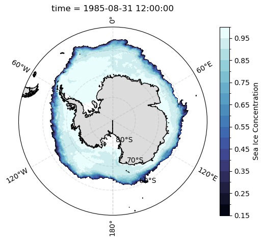
Using cartopy, we can make Polar Stereographic plots of sea ice concentration for a selected month, as follows:
[21]:
def plot_si_conc(data):
    """ A function for plotting tri-polar data"""
    ax = plt.gca()

    # Map the plot boundaries to a circle
    theta = np.linspace(0, 2*np.pi, 100)
    center, radius = [0.5, 0.5], 0.5
    verts = np.vstack([np.sin(theta), np.cos(theta)]).T
    circle = mpath.Path(verts * radius + center)
    ax.set_boundary(circle, transform=ax.transAxes)

    # Add land features and gridlines
    ax.add_feature(cfeature.NaturalEarthFeature('physical', 'land', '50m', edgecolor='black',
                   facecolor = 'gainsboro'), zorder = 2)

    data.plot.contourf(
        transform = ccrs.PlateCarree(),
        x = 'geolon',
        y = 'geolat',
        levels = np.arange(0.15, 1.05, 0.05),
        cmap = cmo.ice,
        cbar_kwargs = {
            'label':'Sea Ice Concentration'
        }
    )

    gl = ax.gridlines(
            draw_labels=True, linewidth=1, color='gray', alpha=0.2, linestyle='--',
            ylocs = np.arange(-80, 81, 10)
        )

    ax.coastlines()
[22]:
def plot_sh_si_conc():
    ax = plt.subplot(projection=ccrs.SouthPolarStereo())

    ax.set_extent([-180, 180, -90, -50], crs=ccrs.PlateCarree())

    plot_si_conc(
        sic.cf.sel(time='1985-08').squeeze('time')
    )

plot_sh_si_conc()
[23]:
def plot_nh_si_conc():
    ax = plt.subplot(projection=ccrs.NorthPolarStereo(central_longitude=-45))

    ax.set_extent([-180, 180, 40, 90], crs=ccrs.PlateCarree())

    plot_si_conc(
        sic.cf.sel(time='1985-02').squeeze('time')
    )

plot_nh_si_conc()
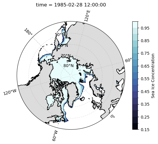
plt.savefig('filepath/filename') function at the end of the cell containing the plot we want to save, as shown below. Note that your filename must contain the file (e.g., pdf, jpeg, png, etc.).plot_sh_si_conc()
plt.savefig('MyFirstSeaIcePlot.png', dpi = 300)