Making Maps with Cartopy¶

Requirements: The conda/analysis3-22.07 (or later) module on the OOD or Gadi (or your own up-to-date cookbook installation).

This tutorial runs through a series of examples that demonstrate how to make maps using data from the COSIMA Cookbook. This tutorial focusses on mapping with Cartopy.

[1]:

%matplotlib inline
%config InlineBackend.figure_format='retina'

import matplotlib.pyplot as plt
import xarray as xr
import numpy as np

import IPython.display
import cmocean as cm
import cartopy.crs as ccrs
import cosima_cookbook as cc

We will use the SST field from a 0.25° resolution experiment as our sample data. These maps should work with any 2D data.

[2]:

session = cc.database.create_session()

experiment = '025deg_jra55v13_iaf_gmredi6'
variable = 'surface_temp'
darray = cc.querying.getvar(experiment, variable, session, frequency='1 monthly', n=-1)
SST = darray.mean('time') - 273.15; # convert from degrees K to degrees C
SST

[2]:

<xarray.DataArray 'surface_temp' (yt_ocean: 1080, xt_ocean: 1440)>
dask.array<sub, shape=(1080, 1440), dtype=float32, chunksize=(540, 720), chunktype=numpy.ndarray>
Coordinates:
  * xt_ocean  (xt_ocean) float64 -279.9 -279.6 -279.4 ... 79.38 79.62 79.88
  * yt_ocean  (yt_ocean) float64 -81.08 -80.97 -80.87 ... 89.74 89.84 89.95

Vanilla `.plot()`¶

You can always make a vanilla plot of this data using xarray…

[3]:

SST.plot();

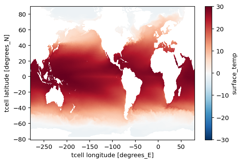
../_images/Tutorials_Making_Maps_with_Cartopy_5_0.png

…, but this doesn’t look that appealing. Or, let’s just make a subjective remark: it doesn’t seem publication-worthy. :)

Also, note that there is (objectively) noticable distortion in the tripole region, i.e., north of 65°N. (For example, with the current plate-tectonics configuration, Canada does not touches the North Pole as the figure might imply.)

Using Cartopy¶

Instead, let’s plot the same data with cartopy. This example uses the Robinson global projection – but note that key argument in the plot function: transform=ccrs.PlateCarree() – which is needed every time you plot something with cartopy. (Confusingly, you could also use a PlateCarree projection, not to be confused with the transformation …)

[4]:

plt.figure(figsize=(8, 4))
ax = plt.axes(projection=ccrs.Robinson())

SST.plot(ax=ax,
         x='xt_ocean', y='yt_ocean',
         transform=ccrs.PlateCarree(),
         vmin=-2, vmax=30, extend='both',
         cmap=cm.cm.thermal)

ax.coastlines();

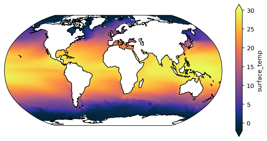
../_images/Tutorials_Making_Maps_with_Cartopy_8_0.png

You can see that this looks a little better.

Colouring in the land¶

Say, for example, we don’t like such a huge colorbar. Also, say we’d prefer the land colour to be something other than white. These details can be dealt with by doing something like the following.

Let’s first colour the land.

[5]:

import cartopy.feature as cft

land_50m = cft.NaturalEarthFeature('physical', 'land', '50m',
                                   edgecolor='black', facecolor='papayawhip', linewidth=0.5)

[6]:

plt.figure(figsize=(8, 4))
ax = plt.axes(projection=ccrs.Robinson())

SST.plot.pcolormesh(ax=ax,
                    x='xt_ocean', y='yt_ocean',
                    transform=ccrs.PlateCarree(),
                    vmin=-2, vmax=30, extend='both',
                    cmap=cm.cm.thermal)

ax.coastlines(resolution='50m')
ax.add_feature(land_50m);

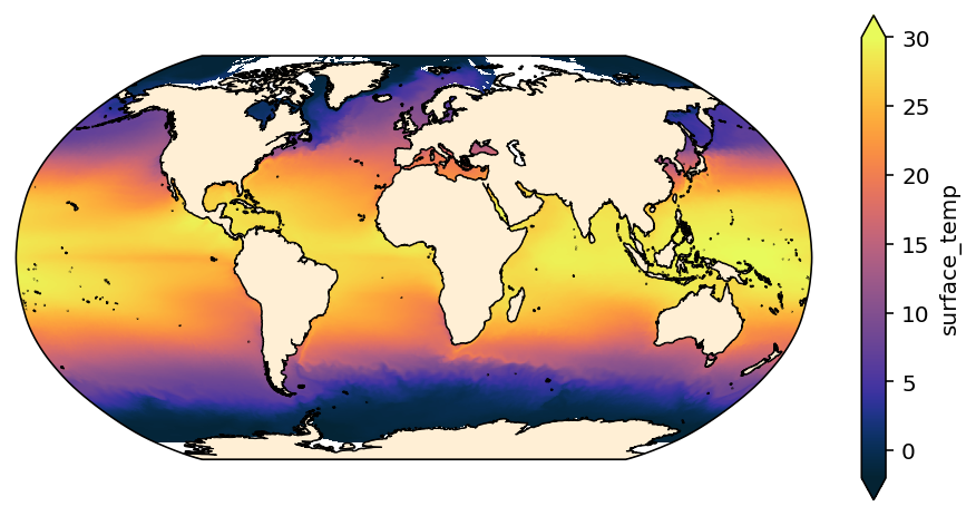
../_images/Tutorials_Making_Maps_with_Cartopy_12_0.png

However, there is still a glitch in this plot – because data in the tripole region is distorted. This occurs because the 1D coordinates xt_ocean and yt_ocean are actually incorrect in the tripole region.

Fixing the tripole¶

Instead, we need to plot with the 2D arrays of x and y locations – geolon_t and geolat_t which we save as static data from each run.

We load geolon_t and geolat_t and assign these 2D-arrays as coordinates on our data array.

[7]:

geolon_t = cc.querying.getvar(experiment, 'geolon_t', session, n=-1)
geolat_t = cc.querying.getvar(experiment, 'geolat_t', session, n=-1)

SST = SST.assign_coords({'geolon_t': geolon_t, 'geolat_t': geolat_t})
SST

[7]:

<xarray.DataArray 'surface_temp' (yt_ocean: 1080, xt_ocean: 1440)>
dask.array<sub, shape=(1080, 1440), dtype=float32, chunksize=(540, 720), chunktype=numpy.ndarray>
Coordinates:
  * xt_ocean  (xt_ocean) float64 -279.9 -279.6 -279.4 ... 79.38 79.62 79.88
  * yt_ocean  (yt_ocean) float64 -81.08 -80.97 -80.87 ... 89.74 89.84 89.95
    geolat_t  (yt_ocean, xt_ocean) float32 dask.array<chunksize=(540, 720), meta=np.ndarray>
    geolon_t  (yt_ocean, xt_ocean) float32 dask.array<chunksize=(540, 720), meta=np.ndarray>

[8]:

fig = plt.figure(figsize=(8, 4))

ax = plt.axes(projection=ccrs.Robinson())

ax.coastlines(resolution='50m')
ax.add_feature(land_50m)
ax.gridlines(draw_labels=False)

SST.plot.contourf(ax=ax,
                  x='geolon_t', y='geolat_t',
                  levels=33, vmin=-2, vmax=30,
                  extend='both',
                  cmap=cm.cm.thermal,
                  transform=ccrs.PlateCarree(),
                  cbar_kwargs = {'label': 'SST (°C)',
                                 'fraction': 0.03,
                                 'aspect': 15,
                                 'shrink': 0.7})

plt.title('Time-mean Sea Surface Temperature');

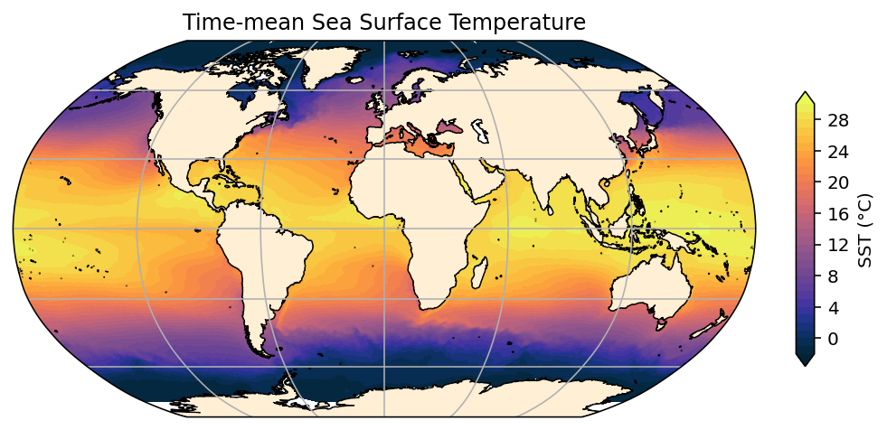
../_images/Tutorials_Making_Maps_with_Cartopy_15_0.png

OK, so that’s a bit better. We also tweaked the colorbar using cbar_kwargs.

But you may have noticed that we had to use contourf to make this map: we can’t use just .plot (which fallsback to pcolormesh) in this instance, because geolon_t and geolat_t we loaded via, e.g.,

cc.querying.getvar(experiment, 'geolat_t', session, n=-1)

are masked arrays and pcolormesh can’t cope with underfined coordinates. (To convince yourself try out SST.plot(x='geolon_t', y='geolat_t').) Our options here are:

Try contourf instead - it should work;
Use pcolor, noting that this is sometimes very slow;
Read in the 2D longitude/latitude coordinates from a file that we prepared earlier …

So to demonstrate the last option here we first drop the masked coordinates drom our data array:

[9]:

SST = SST.drop({'geolon_t', 'geolat_t'})
SST

[9]:

<xarray.DataArray 'surface_temp' (yt_ocean: 1080, xt_ocean: 1440)>
dask.array<sub, shape=(1080, 1440), dtype=float32, chunksize=(540, 720), chunktype=numpy.ndarray>
Coordinates:
  * xt_ocean  (xt_ocean) float64 -279.9 -279.6 -279.4 ... 79.38 79.62 79.88
  * yt_ocean  (yt_ocean) float64 -81.08 -80.97 -80.87 ... 89.74 89.84 89.95

And then load the unmasked ones.

[10]:

# these lon/lat arrays are NOT masked
geolon_t = xr.open_dataset('/g/data/ik11/grids/ocean_grid_025.nc').geolon_t
geolat_t = xr.open_dataset('/g/data/ik11/grids/ocean_grid_025.nc').geolat_t

SST = SST.assign_coords({'geolat_t': geolat_t, 'geolon_t': geolon_t})
SST

[10]:

<xarray.DataArray 'surface_temp' (yt_ocean: 1080, xt_ocean: 1440)>
dask.array<sub, shape=(1080, 1440), dtype=float32, chunksize=(540, 720), chunktype=numpy.ndarray>
Coordinates:
  * xt_ocean  (xt_ocean) float64 -279.9 -279.6 -279.4 ... 79.38 79.62 79.88
  * yt_ocean  (yt_ocean) float64 -81.08 -80.97 -80.87 ... 89.74 89.84 89.95
    geolon_t  (yt_ocean, xt_ocean) float32 -279.9 -279.6 -279.4 ... 80.0 80.0
    geolat_t  (yt_ocean, xt_ocean) float32 -81.08 -81.08 -81.08 ... 65.13 65.03

[11]:

plt.figure(figsize=(8, 4))
ax = plt.axes(projection=ccrs.Robinson())

ax.coastlines(resolution='50m')
ax.add_feature(land_50m)
ax.gridlines(draw_labels=False)

SST.plot(ax=ax,
         x='geolon_t', y='geolat_t',
         transform=ccrs.PlateCarree(),
         vmin=-2, vmax=30, extend='both',
         cmap=cm.cm.thermal,
         cbar_kwargs = {'label': 'SST (°C)',
                        'fraction': 0.03,
                        'aspect': 15,
                        'shrink': 0.7})

plt.title('Time-mean Sea Surface Temperature');

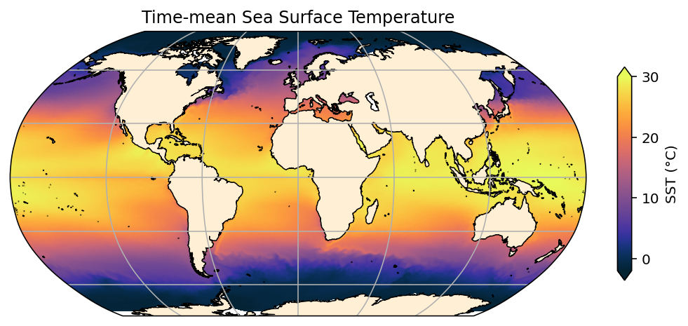
../_images/Tutorials_Making_Maps_with_Cartopy_21_0.png

This is about as good as we can get. Note that there are some mismatches between the coastlines in the model and reality, principally around Antarctica and the Canadian Archipelago. Also, note that the ocean_grid_025.nc file used here will only work for 0.25° resolution cases - check to see if others are available.

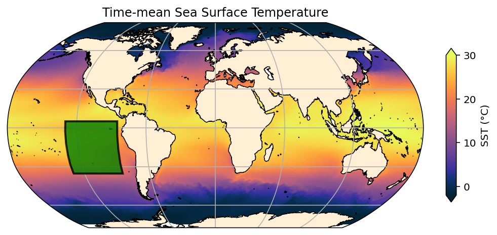
Mark a region¶

Sometimes we want to mark a particular region that our analysis is foccused on. We can do that using matplotlib.patches.

[12]:

import matplotlib.patches as mpatches

plt.figure(figsize=(8, 4))
ax = plt.axes(projection=ccrs.Robinson())

ax.coastlines(resolution='50m')
ax.add_feature(land_50m)
ax.gridlines(draw_labels=False)

SST.plot(ax=ax,
         x='geolon_t', y='geolat_t',
         transform=ccrs.PlateCarree(),
         vmin=-2, vmax=30, extend='both',
         cmap=cm.cm.thermal,
         cbar_kwargs = {'label': 'SST (°C)',
                        'fraction': 0.03,
                        'aspect': 15,
                        'shrink': 0.7})

plt.title('Time-mean Sea Surface Temperature')

ax.add_patch(mpatches.Rectangle(xy=[-130, -35],      # the location of the bottom-left corner of the rectangle
                                width=45, height=40, # the width and height of the rectange (in degrees)
                                facecolor='green',
                                edgecolor='black',
                                linewidth=2,
                                alpha=0.8,
                                fill=True,
                                zorder=3,            # brings the patch in front
                                transform=ccrs.PlateCarree()));

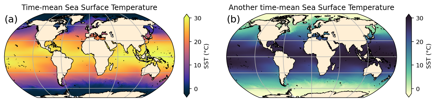
../_images/Tutorials_Making_Maps_with_Cartopy_24_0.png

Subplots¶

It can be a bit tricky to use Cartopy with subplots. Here’s an example:

[13]:

fig, axes = plt.subplots(ncols = 2, subplot_kw={'projection': ccrs.Robinson()}, figsize = (12, 8))

cbar_kwargs = {'label': 'SST (°C)',
               'fraction': 0.03,
               'aspect': 15,
               'shrink': 0.7}

SST.plot(ax=axes[0],
         x='geolon_t', y='geolat_t',
         transform=ccrs.PlateCarree(),
         vmin=-2, vmax=30, extend='both',
         cmap=cm.cm.thermal,
         cbar_kwargs=cbar_kwargs)

SST.plot(ax=axes[1],
         x='geolon_t', y='geolat_t',
         transform=ccrs.PlateCarree(),
         vmin=-2, vmax=30, extend='both',
         cmap=cm.cm.deep,
         cbar_kwargs=cbar_kwargs)

import string

# add features and label panels
for n, ax in enumerate(axes):
    # features
    ax.coastlines(resolution='50m')
    ax.add_feature(land_50m)
    ax.gridlines(draw_labels=False)

    # subplot labels
    ax.text(0, 0.9, '('+string.ascii_lowercase[n]+')', transform=ax.transAxes, size=16)

axes[0].set_title('Time-mean Sea Surface Temperature')
axes[1].set_title('Another time-mean Sea Surface Temperature');

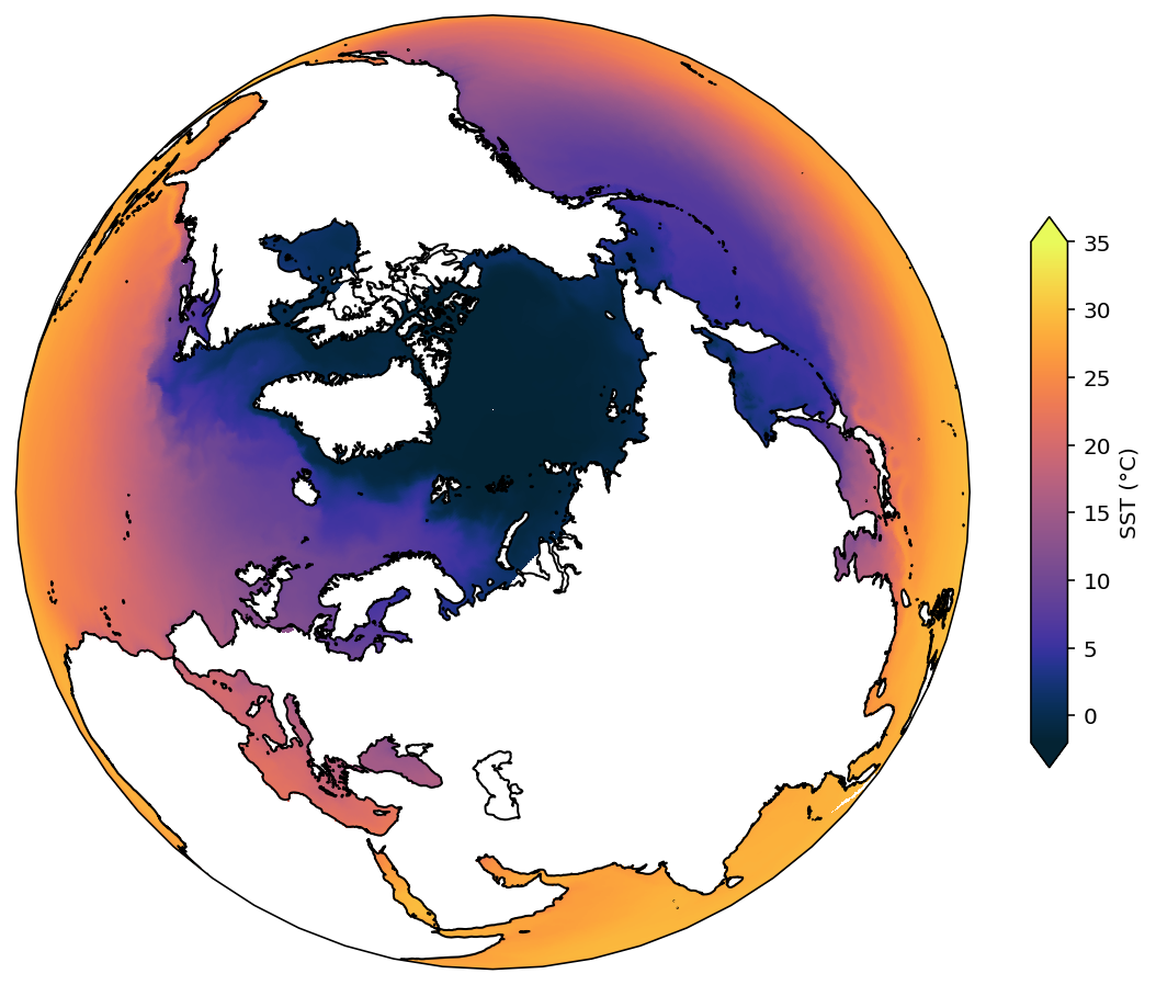
../_images/Tutorials_Making_Maps_with_Cartopy_26_0.png

Projections¶

Here are a few interesting projections you can use with cartopy that might be useful for other applications. Note that if you decide to use a map region which extends north of 65°N, you should use the 2D coordinte files as per above.

[14]:

projection = ccrs.Orthographic(central_latitude=80, central_longitude=50)

plt.figure(figsize=(10, 8))
ax = plt.axes(projection=projection)

ax.coastlines(resolution='50m');

SST.plot(x='geolon_t', y='geolat_t',
         transform=ccrs.PlateCarree(),
         vmin=-2, vmax=35, extend='both',
         cmap=cm.cm.thermal,
         cbar_kwargs = {'label': 'SST (°C)',
                        'fraction': 0.03,
                        'aspect': 15,
                        'shrink': 0.7});

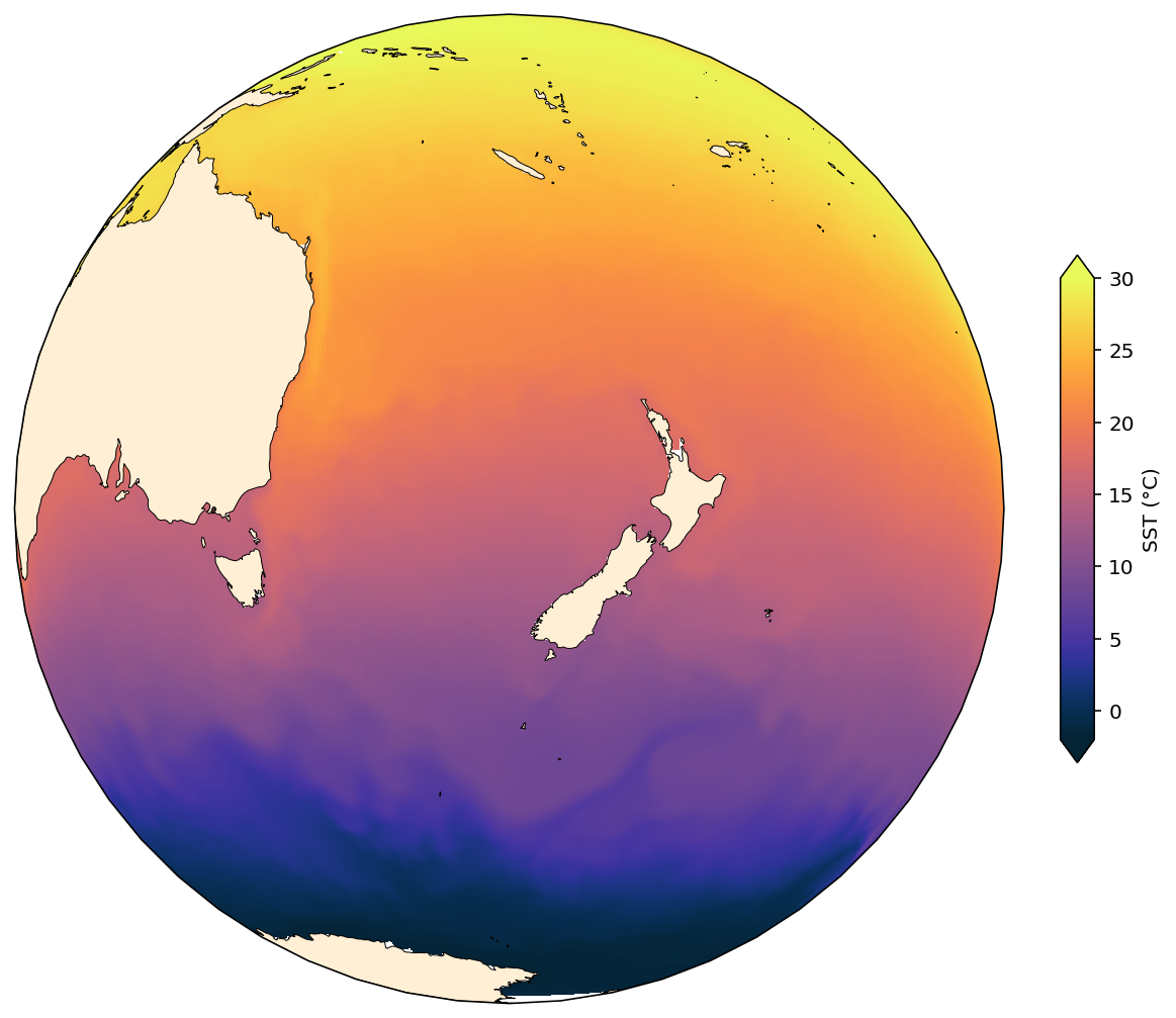
../_images/Tutorials_Making_Maps_with_Cartopy_28_0.png

Near Sided Perspective¶

[15]:

projection = ccrs.NearsidePerspective(central_longitude=165.0, central_latitude=-40.0, satellite_height=2500000)

plt.figure(figsize=(10, 9))
ax = plt.axes(projection=projection)

ax.add_feature(land_50m)

SST.plot(x='geolon_t', y='geolat_t',
         transform=ccrs.PlateCarree(),
         vmin=-2, vmax=30, extend='both',
         cmap=cm.cm.thermal,
         cbar_kwargs = {'label': 'SST (°C)',
                        'fraction': 0.03,
                        'aspect': 15,
                        'shrink': 0.7});

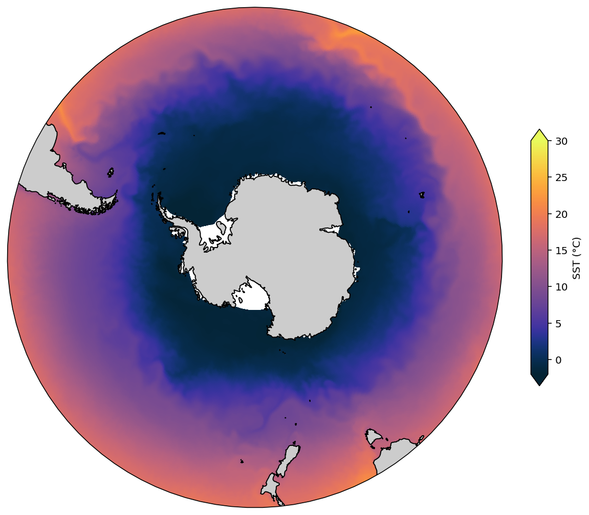
../_images/Tutorials_Making_Maps_with_Cartopy_30_0.png

South Polar Stereo¶

Note that this plot, by default, shows the entire globe, which undermines the area of the South Pole region. So, to enhance our beloved Southern Ocean we have to cut an area of the figure to focus down on it.

[16]:

projection = ccrs.SouthPolarStereo()

plt.figure(figsize=(10, 9))
ax = plt.axes(projection=projection)

ax.set_extent([-280, 80, -80, -35], crs=ccrs.PlateCarree())
ax.add_feature(land_50m, color=[0.8, 0.8, 0.8])
ax.coastlines(resolution='50m')

# Compute a circle in axes coordinates, which we can use as a boundary
# for the map. We can pan/zoom as much as we like - the boundary will be
# permanently circular.

import matplotlib.path as mpath

theta = np.linspace(0, 2*np.pi, 100)
center, radius = [0.5, 0.5], 0.5
verts = np.vstack([np.sin(theta), np.cos(theta)]).T
circle = mpath.Path(verts * radius + center)
ax.set_boundary(circle, transform=ax.transAxes)

SST.plot(x='geolon_t', y='geolat_t',
         transform=ccrs.PlateCarree(),
         vmin=-2, vmax=30, extend='both',
         cmap=cm.cm.thermal,
         cbar_kwargs = {'label': 'SST (°C)',
                        'fraction': 0.03,
                        'aspect': 15,
                        'shrink': 0.7});

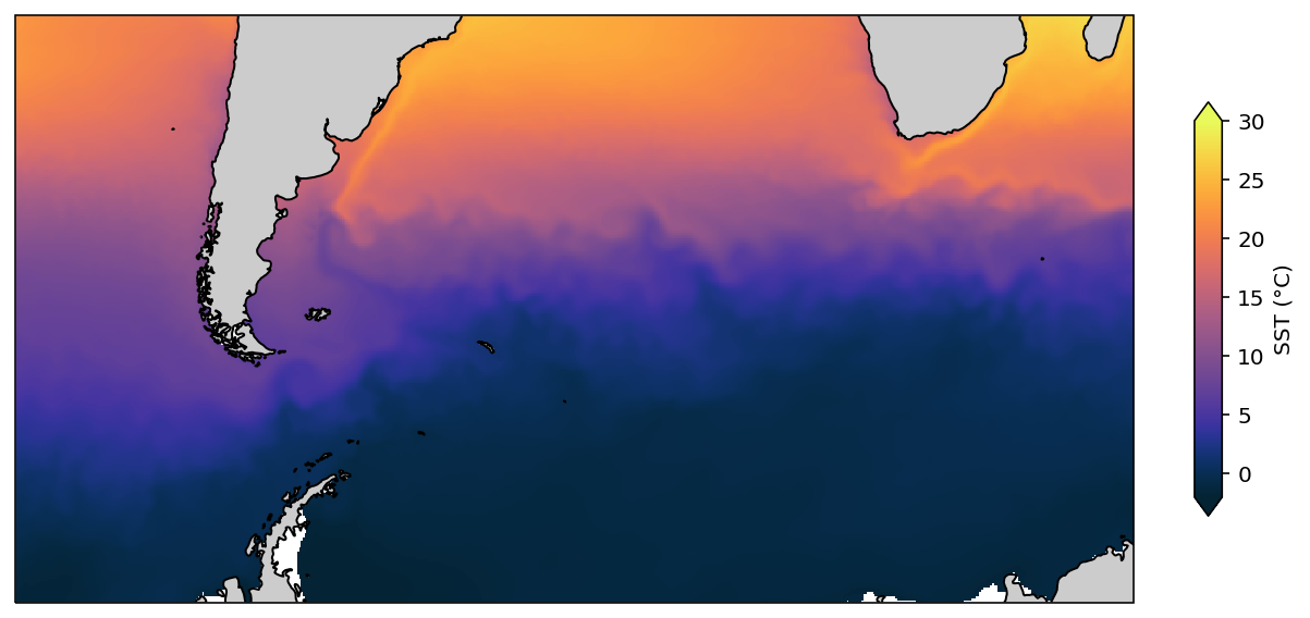
../_images/Tutorials_Making_Maps_with_Cartopy_32_0.png

Mercator regional plot¶

[17]:

projection = ccrs.Mercator(central_longitude=0.0, min_latitude=-70.0, max_latitude=-20.0)

plt.figure(figsize=(10, 5))
ax = plt.axes(projection=projection)

ax.set_extent([-100, 50, -70, -20], crs=ccrs.PlateCarree())
ax.add_feature(land_50m, color=[0.8, 0.8, 0.8])
ax.coastlines(resolution='50m')

SST.plot(x='geolon_t', y='geolat_t',
         transform=ccrs.PlateCarree(),
         vmin=-2, vmax=30, extend='both',
         cmap=cm.cm.thermal,
         cbar_kwargs = {'label': 'SST (°C)',
                        'fraction': 0.03,
                        'aspect': 15,
                        'shrink': 0.7});

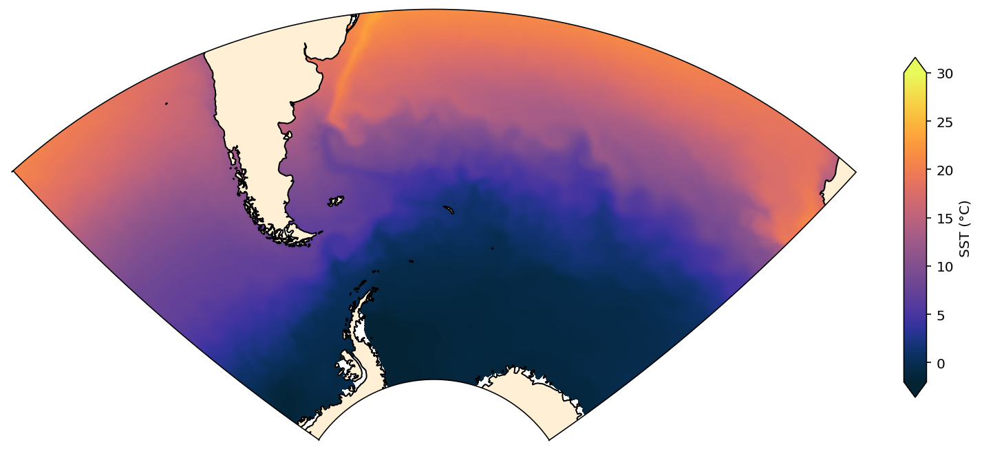
../_images/Tutorials_Making_Maps_with_Cartopy_34_0.png

Sector map¶

This map shows a sector of the Southern Ocean. It involves a Stereographic projection and a fairly complicated cutout to set the boundary of the map, but gives a nice result.

[18]:

def make_boundary_path(longitudes, latitudes):
    """
    Return a path around boundary to create a sector map, then cut it out given
    longitudes and latitudes.
    """
    boundary_path = np.array([longitudes[-1, :], latitudes[-1, :]])
    boundary_path = np.append(boundary_path, np.array([longitudes[::-1, -1], latitudes[::-1, -1]]), axis=1)
    boundary_path = np.append(boundary_path, np.array([longitudes[1, ::-1],  latitudes[1, ::-1]]), axis=1)
    boundary_path = np.append(boundary_path, np.array([longitudes[:, 1],     latitudes[:, 1]]), axis=1)
    boundary_path = mpath.Path(np.swapaxes(boundary_path, 0, 1))

    return boundary_path

[19]:

midlon = -40
maxlon = midlon + 60
minlon = midlon - 60
minlat = -75
maxlat = -30
midlat = (minlat + maxlat)/2

projection=ccrs.Stereographic(central_longitude=midlon, central_latitude=midlat)

fig = plt.figure(figsize=(12, 6.5))
ax = plt.axes(projection=projection)

ax.add_feature(land_50m)
ax.coastlines(resolution='50m')
ax.set_extent([minlon, maxlon, minlat, maxlat], crs=ccrs.PlateCarree())

lons = geolon_t.sel({'xt_ocean': slice(minlon, maxlon), 'yt_ocean': slice(minlat, maxlat)})
lats = geolat_t.sel({'xt_ocean': slice(minlon, maxlon), 'yt_ocean': slice(minlat, maxlat)})
boundary_path = make_boundary_path(lons, lats)
ax.set_boundary(boundary_path, transform=ccrs.PlateCarree())

SST.plot(x='geolon_t', y='geolat_t',
         transform=ccrs.PlateCarree(),
         vmin=-2, vmax=30, extend='both',
         cmap=cm.cm.thermal,
         cbar_kwargs = {'label': 'SST (°C)',
                        'fraction': 0.03,
                        'aspect': 15,
                        'shrink': 0.7});

../_images/Tutorials_Making_Maps_with_Cartopy_37_0.png

You can see a wider selection of cartopy projections in its documentation: https://scitools.org.uk/cartopy/docs/latest

Making Maps with Cartopy¶

Vanilla `.plot()`¶

Using Cartopy¶

Colouring in the land¶

Fixing the tripole¶

Mark a region¶

Subplots¶

Projections¶

Near Sided Perspective¶

South Polar Stereo¶

Mercator regional plot¶

Sector map¶

COSIMA Recipes

Navigation

Related Topics

Making Maps with Cartopy¶

Vanilla .plot()¶

Using Cartopy¶

Colouring in the land¶

Fixing the tripole¶

Mark a region¶

Subplots¶

Projections¶

Near Sided Perspective¶

South Polar Stereo¶

Mercator regional plot¶

Sector map¶

Vanilla `.plot()`¶