Spatial selection with tripolar ACCESS-OM2 grid
The ACCESS-OM2 model collection utilises a tripolar grid north of 65N to avoid a point of convergence over the ocean at the north pole.
This means any plotting or analysis in this region needs to use 2D curvilinear latitude and longitude coordinates.
This notebook will cover how to use the curvilinear coordinates to select data within latitude and longitude limits, and how to plot data in the tripole region correctly. There is also a full tutorial on plotting with projections.
Below the tripole area it is sufficient to use 1D latitude and longitude coordinates, which are much more convenient to use as they can use the xarray’s sel method with slice notation.
This notebook will also demonstrate how to do this.
The data output from the CICE model component do not have a convenient to use 1D latitude and longitude coordinates. As the ice and ocean models share a grid the coordinates from each model can be used interchangeably with the other. A method to add 1D latitude and longitude coordinates to an ice `xarray.DataArray <http://xarray.pydata.org/en/stable/generated/xarray.DataArray.html>`__ is also demonstrated.
[1]:
import cosima_cookbook as cc
import matplotlib.pyplot as plt
import xarray as xr
import numpy as np
import cartopy.crs as ccrs
Load data
Open a database session
[2]:
session = cc.database.create_session()
The specific experiment does not matter a great deal. This is the main IAF control run with JRA55 v1.4 forcing
[3]:
expt = '01deg_jra55v140_iaf'
Load the 1D latitude/longitude variables from the ocean data to use them with ice data. The dimensions are renamed to match the required dimension in the ice data
[4]:
yt_ocean = cc.querying.getvar(expt, 'yt_ocean', session, 'ocean-2d-geolat_t.nc', n=1).rename({'yt_ocean': 'latitude'})
xt_ocean = cc.querying.getvar(expt, 'xt_ocean', session, 'ocean-2d-geolat_t.nc', n=1).rename({'xt_ocean': 'longitude'})
Both the ocean and the ice output variables have masked curvilinear coordinates, which means there are missing values for the coordinates over land. These variables are not suitable for plotting with cartopy. A full curvilinear grid is available from the CICE model input grid:
[5]:
ice_grid = xr.open_dataset('/g/data/ik11/inputs/access-om2/input_eee21b65/cice_01deg/grid.nc')
Extract the full curvilinear coordinates, from the ice grid. Note that these are in radians and so neeed to converted to degrees, and again the dimensions are renamed to match the dataset to which they will be added:
[6]:
geolon_t = np.degrees(ice_grid.tlon.rename({'nx': 'longitude', 'ny': 'latitude'}))
geolat_t = np.degrees(ice_grid.tlat.rename({'nx': 'longitude', 'ny': 'latitude'}))
Load an ice variable to use as an example dataset. In this case only the first 12 months for purposes of illustration.
[7]:
aice_m = cc.querying.getvar(expt, 'aice_m', session, n=12)
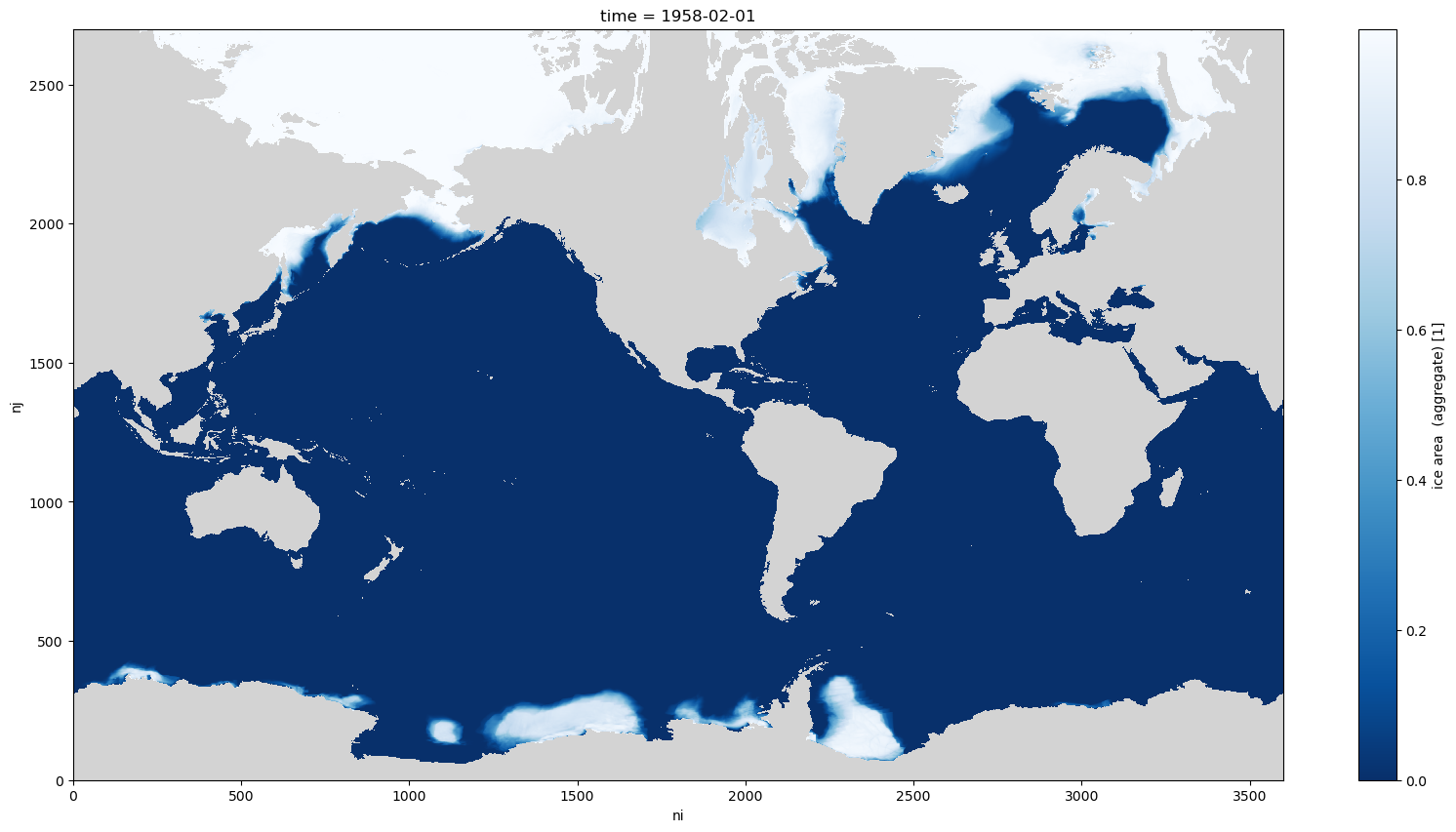
Printing the variable shows it has non-informative dimension names and no CF coordinate variables. As a result when the first time slice is plotted there is no useful units automatically added to the plot.
[8]:
aice_m
[8]:
<xarray.DataArray 'aice_m' (time: 12, nj: 2700, ni: 3600)>
dask.array<concatenate, shape=(12, 2700, 3600), dtype=float32, chunksize=(1, 675, 900), chunktype=numpy.ndarray>
Coordinates:
  * time     (time) datetime64[ns] 1958-02-01 1958-03-01 ... 1959-01-01
    TLON     (nj, ni) float32 dask.array<chunksize=(675, 900), meta=np.ndarray>
    TLAT     (nj, ni) float32 dask.array<chunksize=(675, 900), meta=np.ndarray>
    ULON     (nj, ni) float32 dask.array<chunksize=(675, 900), meta=np.ndarray>
    ULAT     (nj, ni) float32 dask.array<chunksize=(675, 900), meta=np.ndarray>
Dimensions without coordinates: nj, ni
Attributes:
    units:          1
    long_name:      ice area  (aggregate)
    cell_measures:  area: tarea
    cell_methods:   time: mean
    time_rep:       averaged
    ncfiles:        ['/g/data/cj50/access-om2/raw-output/access-om2-01/01deg_...
    contact:        Andrew Kiss
    email:          andrew.kiss@anu.edu.au
    created:        2020-06-09
    description:    0.1 degree ACCESS-OM2 global model configuration under in...
notes: Source code: https://github.com/COSIMA/access-om2 License...Define colormap for plotting. There are two options here depending on your preference. 1. Option 1: Standard ice colormap from cmocean 2. Option 2: Colormap from dark blue (open ocean) to white (100% sea ice cover)
[9]:
def ice_cmap(colormap):
    from palettable.colorbrewer.sequential import Blues_9_r
    import cmocean as cmo

    if colormap == 'Option 1':
        cmap = cmo.cm.ice
        cmap.set_bad('lightgrey') # set color for land
    else:
        cmap = Blues_9_r.mpl_colormap
        cmap.set_bad('lightgrey') # set color for land

    return cmap
[10]:
colormap = 'Option 2'
cmap = ice_cmap(colormap)
cmap
[10]:

[ ]:
aice_m.isel(time=0).plot(aspect=2,size=10, cmap=cmap);
Add spatial coordinates
To improve usability CF compatible spatial coordinates from the ocean data loaded above can be added to the ice data.
The unintuitive dimensions are renamed, and importantly match the dimension names chosen for the coordinates. The coordinates loaded above are added to the DataArray, and saved in a new variable, aice_m_coords.
[ ]:
aice_m_coords = aice_m.rename({'nj':'latitude',
                               'ni':'longitude'}).assign_coords({'latitude': yt_ocean,
                                                                 'longitude': xt_ocean,
                                                                 'geolat_t': geolat_t,
                                                                 'geolon_t': geolon_t})
aice_m_coords
<xarray.DataArray 'aice_m' (time: 12, latitude: 2700, longitude: 3600)>
dask.array<concatenate, shape=(12, 2700, 3600), dtype=float32, chunksize=(1, 675, 900), chunktype=numpy.ndarray>
Coordinates:
  * time       (time) datetime64[ns] 1958-02-01 1958-03-01 ... 1959-01-01
    TLON       (latitude, longitude) float32 dask.array<chunksize=(675, 900), meta=np.ndarray>
    TLAT       (latitude, longitude) float32 dask.array<chunksize=(675, 900), meta=np.ndarray>
    ULON       (latitude, longitude) float32 dask.array<chunksize=(675, 900), meta=np.ndarray>
    ULAT       (latitude, longitude) float32 dask.array<chunksize=(675, 900), meta=np.ndarray>
  * latitude   (latitude) float64 -81.11 -81.07 -81.02 ... 89.89 89.94 89.98
  * longitude  (longitude) float64 -279.9 -279.8 -279.7 ... 79.75 79.85 79.95
    geolat_t   (latitude, longitude) float64 -81.11 -81.11 ... 65.06 65.02
    geolon_t   (latitude, longitude) float64 -279.9 -279.8 -279.7 ... 80.0 80.0
Attributes:
    units:          1
    long_name:      ice area  (aggregate)
    cell_measures:  area: tarea
    cell_methods:   time: mean
    time_rep:       averaged
    ncfiles:        ['/g/data/cj50/access-om2/raw-output/access-om2-01/01deg_...
    contact:        Andrew Kiss
    email:          andrew.kiss@anu.edu.au
    created:        2020-06-09
    description:    0.1 degree ACCESS-OM2 global model configuration under in...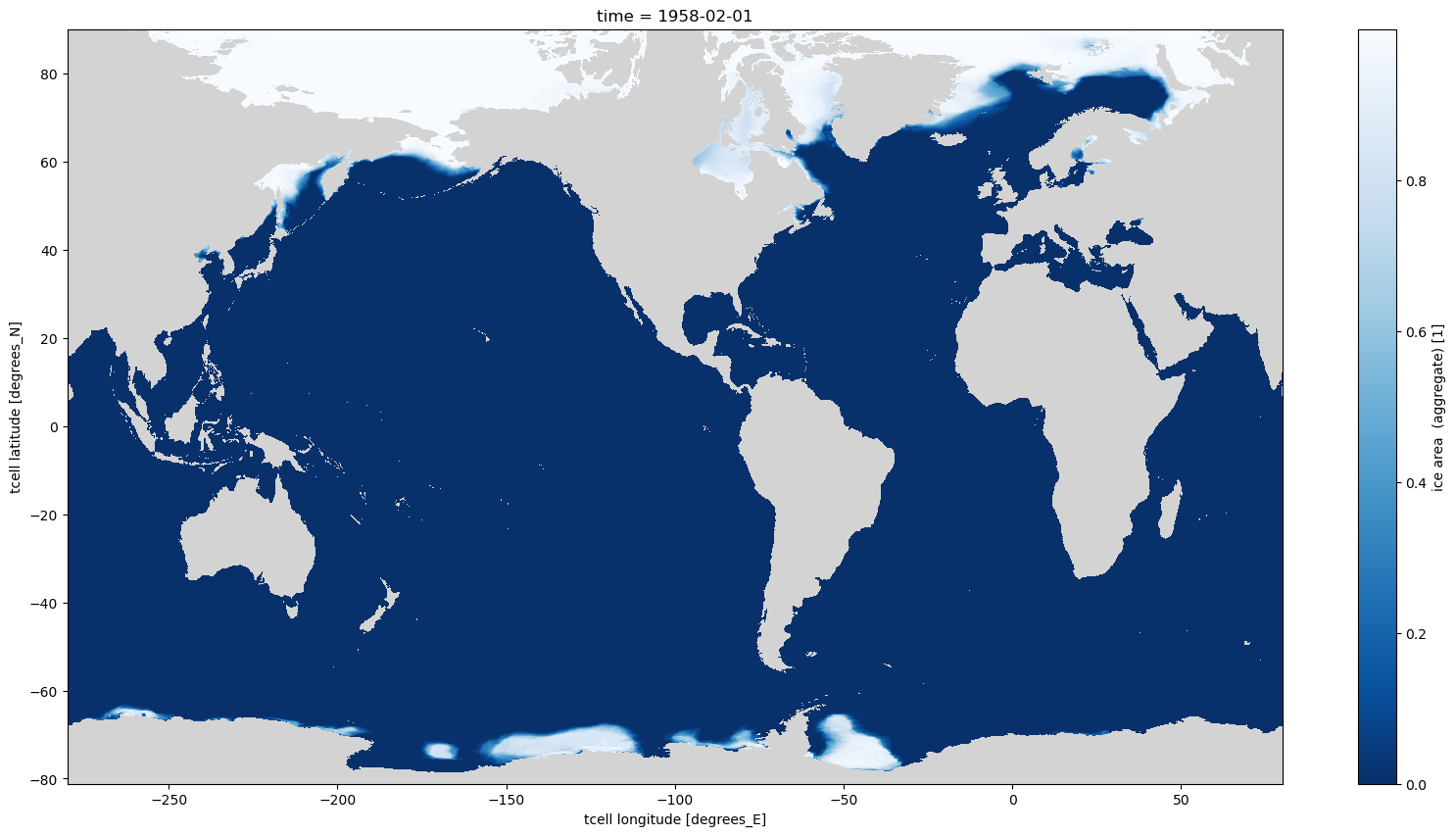
notes: Source code: https://github.com/COSIMA/access-om2 License...Now when the first time slice is plotted there are informative axes as there are now CF compliant dimensions latitude and longitude.
[13]:
aice_m_coords.isel(time=0).plot(aspect=2, size=10, cmap=cmap);
Selection using sel and slice
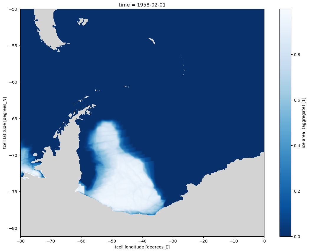
Also selection using slices of latitude and longitude are easy using these new dimensions. e.g. selecting the Weddell Sea in Antarctica
[14]:
aice_m_coords.isel(time=0).sel(longitude=slice(-80, 0), latitude=slice(None, -50)).plot(size=10, cmap=cmap);
The same data can also be plotted and projected using cartopy which works fine using the 1D latitude and longitude coordinates as these are correct for all values south of 65N, so all of the Southern Hemisphere.
[15]:
fig = plt.figure(figsize=(14, 8))
ax = plt.axes(projection=ccrs.Orthographic(-40, -90))
ax.coastlines()
ax.gridlines()
aice_m_coords.isel(time=0).sel(longitude=slice(-80, 0),
                               latitude=slice(None, -50)).plot(ax=ax,
                                                               transform=ccrs.PlateCarree(),
                                                               cmap=cmap);
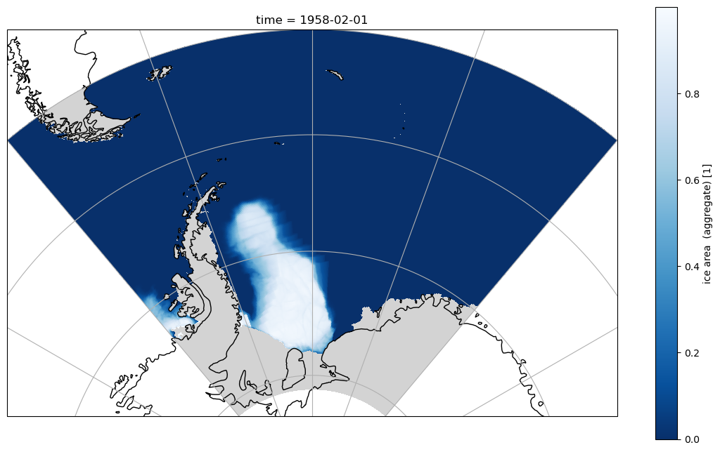
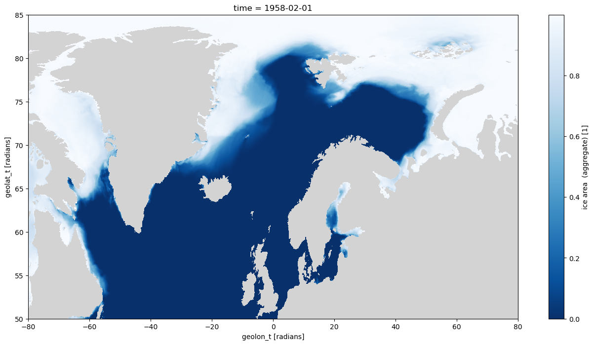
Simple sel with slice can also be used to select areas in the northern hemisphere, but they appear distorted as this area is in the tripole, so the 1D latitude and longitude variables are not correct
[16]:
aice_m_coords.isel(time=0).sel(longitude=slice(-80, 80),
                               latitude=slice(50, 85)).plot(size=8, aspect=2, cmap=cmap);
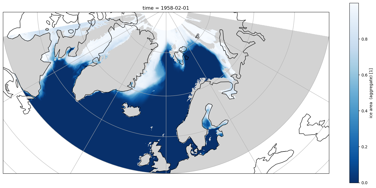
If the same selection is plotted in an Orthographic projection with cartopy it is obvious that land/sea boundaries are not correct, and artefacts from the tripole are visible
[17]:
fig = plt.figure(figsize=(18, 8))
ax = plt.axes(projection=ccrs.Orthographic(0, 90))
ax.coastlines()
ax.gridlines()
aice_m_coords.isel(time=0).sel(longitude=slice(-80, 80),
                               latitude=slice(50, 85)).plot(ax=ax,
                                                            cmap=cmap,
                                                            transform=ccrs.PlateCarree());
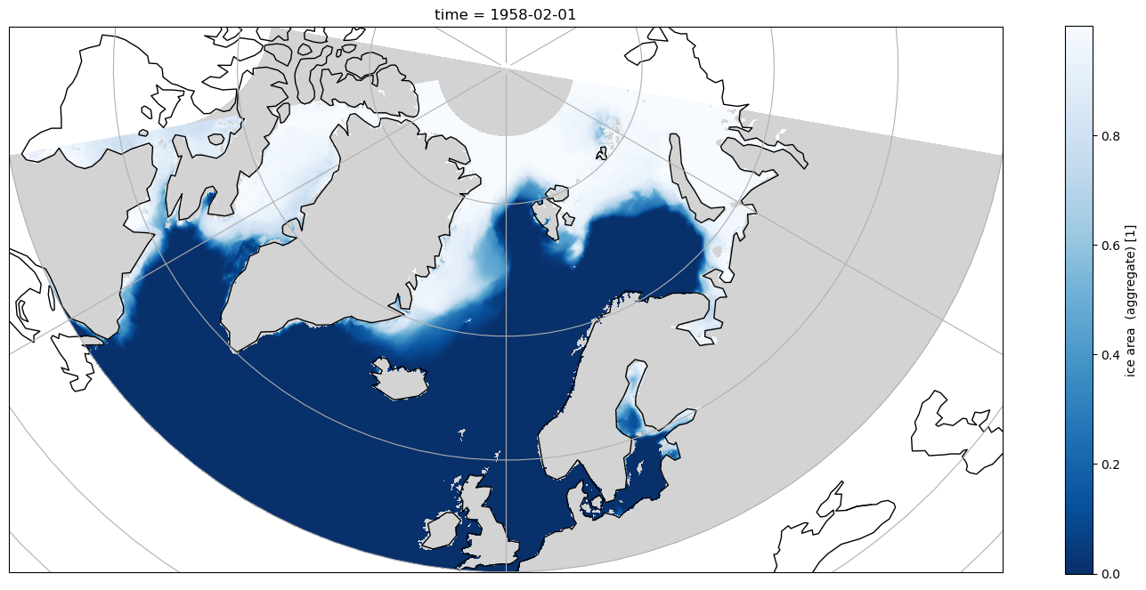
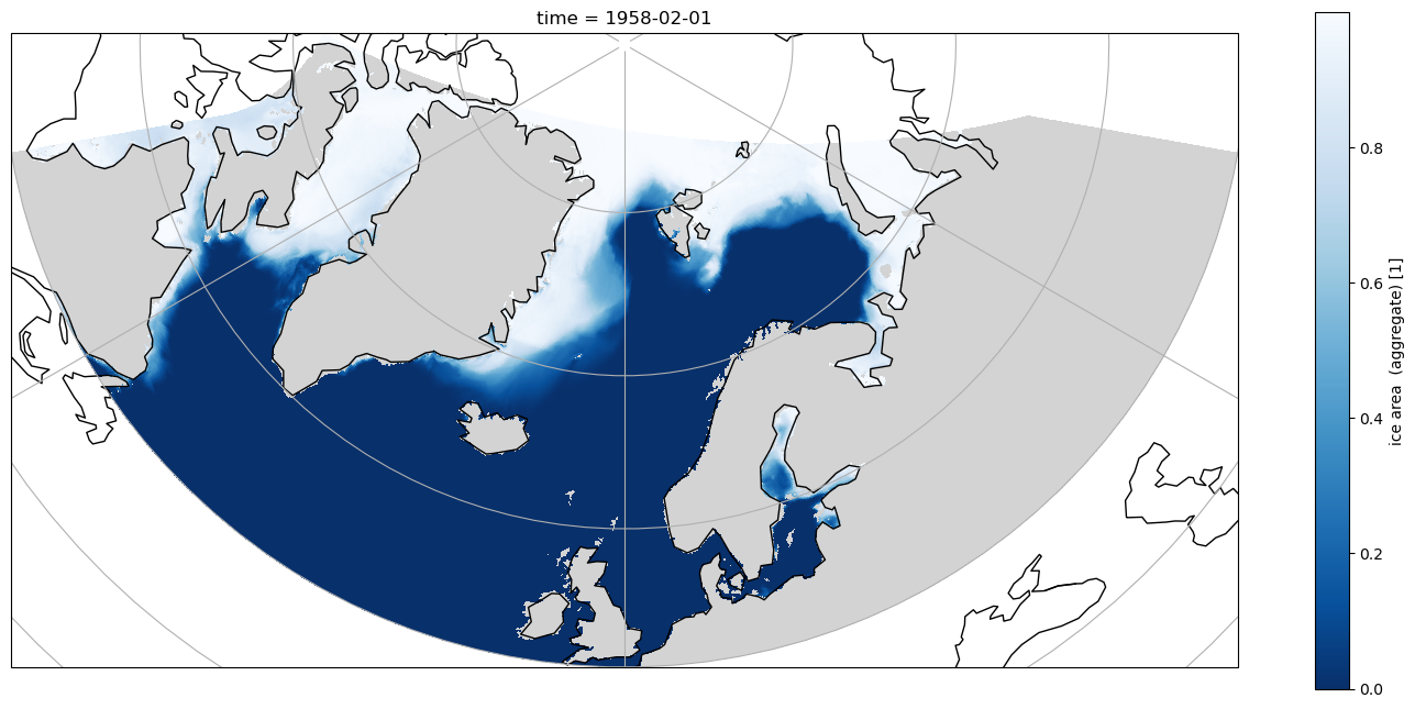
Using the true curvilinear coordinates to plot, the artefacts are removed, and the land/sea registration is correct, but the simple sel using the 1D coordinates means there are not constant lines of latitude or longitude in the selected data.
[18]:
fig = plt.figure(figsize=(18, 8))
ax = plt.axes(projection=ccrs.Orthographic(0,90))
ax.coastlines()
ax.gridlines()
aice_m_coords.isel(time=0).sel(longitude=slice(-80, 80),
                               latitude=slice(50, 85)).plot(ax=ax, cmap=cmap,
                                                            transform=ccrs.PlateCarree(),
                                                            x='geolon_t', y='geolat_t');
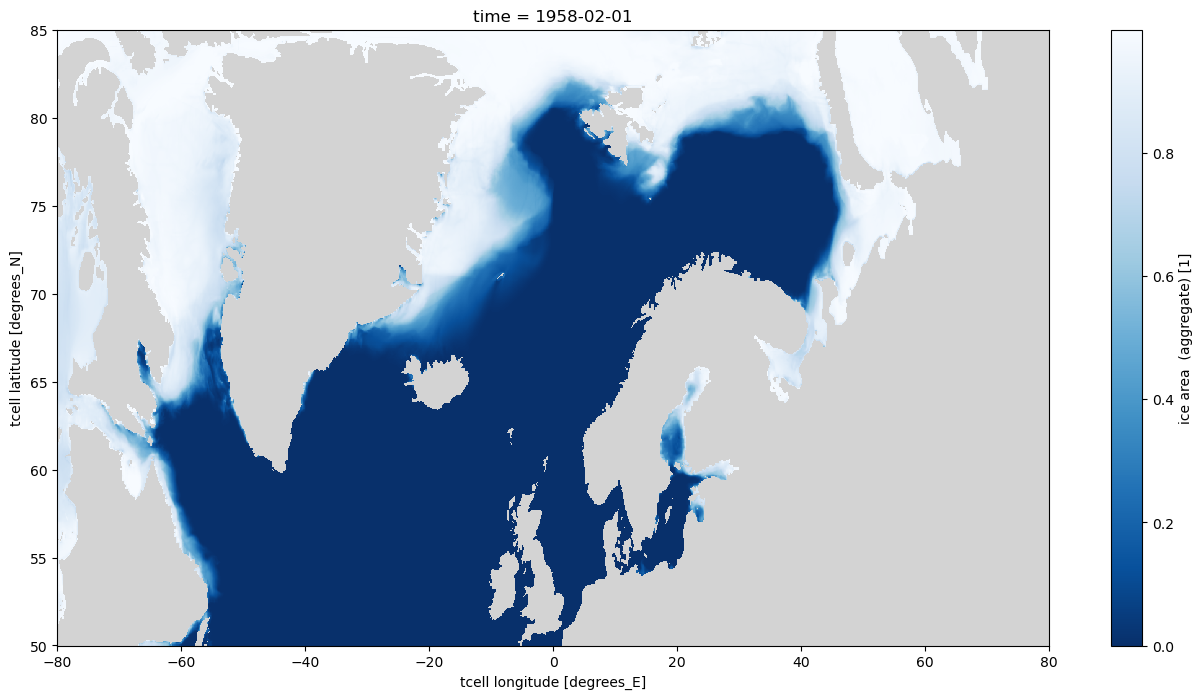
Selection using where
To do proper spatial selection with 2D coordinates in the tripole area it is necessary to use the xarray `where <http://xarray.pydata.org/en/stable/generated/xarray.DataArray.where.html>`__ method, which will mask out the data where the stipulated condition is not met. With drop=True coordinate labels with only False values are removed.
[19]:
aice_m_coords.isel(time=0).where((geolon_t >= -80) &
                                 (geolon_t <= 80) &
                                 (geolat_t >= 50) &
                                 (geolat_t <= 85), drop=True).plot(size=8, aspect=2,
                                                                   x='geolon_t',
                                                                   y='geolat_t',
                                                                   cmap=cmap)
plt.xlim([-80, 80])
plt.ylim([50, 85]);
Now when plotted in Orthographic projection with cartopy the selection is clearly along lines of constant latitude, and the left hand side selection is a constant longitude.
[20]:
fig = plt.figure(figsize=(18, 8))
ax = plt.axes(projection=ccrs.Orthographic(0, 90))
ax.coastlines()
ax.gridlines()
aice_m_coords.isel(time=0).where((aice_m_coords.geolon_t >= -80) &
                                 (aice_m_coords.geolon_t <= 80) &
                                 (aice_m_coords.geolat_t >= 50) &
                                 (aice_m_coords.geolat_t <= 85), drop=True).plot(ax=ax,
                                                                                 transform=ccrs.PlateCarree(),
                                                                                 x='geolon_t',
                                                                                 y='geolat_t',
                                                                                 cmap = cmap);