Calculating pairwise distances between a contour and every grid cell
In this notebook, we will demonstrate how to calculate the distance from every grid cell to the nearest grid cell along a contour. We will demonstrate this by computing the distance from each grid cell in a data array to the sea ice edge. We will use monthly sea ice concentration from ACCESS-OM2-01 over the Southern Ocean to perform these calculations.
i, j.Loading modules
[1]:
import cosima_cookbook as cc
import xarray as xr
import numpy as np
import datetime as dt
from sklearn.neighbors import BallTree
import matplotlib.pyplot as plt
Creating a session in the COSIMA cookbook
[2]:
session = cc.database.create_session()
Accessing ACCESS-OM2-01 data
We will use monthly sea ice outputs from cycle four. For this example, we will load only two months of sea ice data. Note the use of decode_coords = False. This avoids lengthly delays in accessing sea ice data. See more information here.
[3]:
var_ice = cc.querying.getvar('01deg_jra55v140_iaf_cycle4', 'aice_m', session,
                             start_time='1978-01', end_time='1978-03',
                             decode_coords=False)
The sea ice outputs need some processing before we can start our calculations. You can check this example for a guide on how to load and plot sea ice data.
We will follow these processing steps: 1. Correct time dimension values by subtracting 12 hours, 2. Attach the ocean model grid so we can calculate distances.
[4]:
# Loading area_t to get ocean grid
area_t = cc.querying.getvar('01deg_jra55v140_iaf_cycle4', 'area_t', session, n=1)

# Apply time correction so data appears in the middle (12:00) of the day rather than at the beginning of the day (00:00)
var_ice['time'] = var_ice.time.to_pandas() - dt.timedelta(hours = 12)

# Change coordinates so they match ocean dimensions
var_ice.coords['ni'] = area_t['xt_ocean'].values
var_ice.coords['nj'] = area_t['yt_ocean'].values

# Rename coordinate variables so they match ocean data
var_ice = var_ice.rename(({'ni': 'xt_ocean', 'nj': 'yt_ocean'}))

# Subsetting data for the Southern Ocean
var_ice = var_ice.sel(yt_ocean = slice(-80, -45))
var_ice
[4]:
<xarray.DataArray 'aice_m' (time: 3, yt_ocean: 713, xt_ocean: 3600)>
dask.array<getitem, shape=(3, 713, 3600), dtype=float32, chunksize=(1, 270, 360), chunktype=numpy.ndarray>
Coordinates:
  * time      (time) datetime64[ns] 1977-12-31T12:00:00 ... 1978-02-28T12:00:00
  * xt_ocean  (xt_ocean) float64 -279.9 -279.8 -279.7 ... 79.75 79.85 79.95
  * yt_ocean  (yt_ocean) float64 -79.97 -79.93 -79.88 ... -45.18 -45.11 -45.04
Attributes:
    units:          1
    long_name:      ice area  (aggregate)
    coordinates:    TLON TLAT time
    cell_measures:  area: tarea
    cell_methods:   time: mean
    time_rep:       averaged
    ncfiles:        ['/g/data/cj50/access-om2/raw-output/access-om2-01/01deg_...
    contact:        Andrew Kiss
    email:          andrew.kiss@anu.edu.au
    created:        2022-04-27
    description:    0.1 degree ACCESS-OM2 global model configuration under in...
notes: Run configuration and history: https://github.com/COSIMA/...Finding sea ice edge
The sea ice edge is the defined as the northernmost areas where sea ice concentration (SIC) is over \(10\%\). This is a multistep process:
Identify cells where \(\text{SIC} >= 0.1\), classifying them with a value of 1;
Calculate the cumulative sum along latitude;
Apply mask to constrain to only cells with \(\text{SIC} >= 0.1\);
Choose the maximum for each longitude.
We’ll demonstrate this process over the first timestep of data.
[5]:
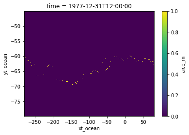
is_ice = var_ice.isel(time=0) >= 0.1
cumulative_ice = is_ice.cumsum(dim='yt_ocean')
ice_edge = (cumulative_ice == cumulative_ice.max('yt_ocean')) * is_ice

ice_edge.plot()
[5]:
<matplotlib.collections.QuadMesh at 0x14c666a25eb0>
Checking results in relation to SIC data
[6]:
var_ice.where(var_ice >= 0.1).isel(time=0).plot()
ice_edge.plot.contour(colors=["red"])
[6]:
<matplotlib.contour.QuadContourSet at 0x14c66488e5b0>
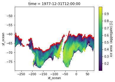
Above we plotted only cells with SIC greater or equal to 0.1. The red line represents the sea ice edge we identified in the previous step. We can be satisfied that we identified the sea ice edge correctly.
Getting coordinate pairs for our entire grid
We will use the latitude and longitude values in our data to create coordinate pairs. We only need to get this information once if we are calculating distances from the same grid.
[7]:
grid_x, grid_y = np.meshgrid(
    var_ice.xt_ocean.values,
    var_ice.yt_ocean.values,
)

# Changing shape so there are two values per row
grid_coords = np.vstack([grid_y.flat, grid_x.flat]).T
grid_coords
[7]:
array([[ -79.96816911, -279.95      ],
       [ -79.96816911, -279.85      ],
       [ -79.96816911, -279.75      ],
       ...,
       [ -45.03607147,   79.75      ],
       [ -45.03607147,   79.85      ],
       [ -45.03607147,   79.95      ]])
Getting coordinate pairs for sea ice edge
We will find the index for the sea ice edge so we can identify the latitude at which the sea ice edge occurs. This will be combined with all longitude values to create the coordinate pairs for the sea ice edge.
Note that this step has to be done once for every time step as the sea ice edge changes over time.
[8]:
# Getting the indices for cell with maximum value along yt_ocean dimension
ice_yt = ice_edge.yt_ocean[ice_edge.argmax(dim='yt_ocean')]
ice_coords = np.vstack([ice_yt, ice_edge.xt_ocean]).T
ice_coords
[8]:
array([[ -61.84325357, -279.95      ],
       [ -61.84325357, -279.85      ],
       [ -61.84325357, -279.75      ],
       ...,
       [ -61.60640174,   79.75      ],
       [ -61.65391774,   79.85      ],
       [ -61.84325357,   79.95      ]])
Using Nearest Neighbours algorithm to calculate distance to closest sea ice edge cell
We will build a data structure called BallTree for our calculations, from the points comprising the sea ice edge. This structure allows us to efficiently query the nearest point within the sea ice edge set to any arbitrary point, according to some kind of metric. Because we’re on a sphere, we use the haversine (great circle)
distance, which also requires that we transform coordinates from degrees to radians. scikit-learn also offers a KDTree for a similar purpose, but this doesn’t support the haversine distance as a metric, so we opt for the ball tree instead.
The advantage of using a data structure like a ball tree is that we trade off slightly more time and memory to construct the tree for more efficient querying. This makes it feasible to query the closest sea ice edge cell to every point on the grid, which may otherwise have excessive time and/or memory requirements for a brute force approach.
[9]:
%%time

# First we set up our Ball Tree. Coordinates must be given in radians.
ball_tree = BallTree(np.deg2rad(ice_coords), metric='haversine')
CPU times: user 1.65 ms, sys: 1.38 ms, total: 3.03 ms
Wall time: 6.81 ms
[10]:
%%time

# The nearest neighbour calculation will give two outputs: distances and indices
# We only need the distances for now, so ignore the second output
distances_radians, _ = ball_tree.query(np.deg2rad(grid_coords), return_distance=True)
CPU times: user 23 s, sys: 0 ns, total: 23 s
Wall time: 23 s
Transforming distance from radians to kilometers
Because the haversine distance operates in terms of radians only, we will need to multiply by the resulting distances by Earth’s radius to get distances in radians. We will also reshape the results so it matches our original grid.
[11]:
distances_km = distances_radians * 6371

distances_t0 = xr.DataArray(
    data=distances_km.reshape(var_ice.yt_ocean.size, -1),
    dims=['yt_ocean', 'xt_ocean'],
    coords={'yt_ocean': var_ice.yt_ocean, 'xt_ocean': var_ice.xt_ocean}
)

distances_t0
[11]:
<xarray.DataArray (yt_ocean: 713, xt_ocean: 3600)>
array([[ 805.00144028,  803.19226827,  801.38249999, ...,  810.42536522,
         808.61799012,  806.81001469],
       [ 806.69292563,  804.88000362,  803.06648432, ...,  812.12809432,
         810.31697234,  808.50524899],
       [ 808.40803346,  806.59143086,  804.77423025, ...,  813.85423949,
         812.03943914,  810.22403667],
       ...,
       [1607.76336769, 1606.55053756, 1605.36467069, ..., 1611.56299844,
        1610.26966326, 1609.00309777],
       [1615.51041181, 1614.30178279, 1613.12003095, ..., 1619.29692977,
        1618.0080497 , 1616.74585538],
       [1623.26793377, 1622.06347241, 1620.88580274, ..., 1627.04144284,
        1625.75698268, 1624.4991249 ]])
Coordinates:
  * yt_ocean  (yt_ocean) float64 -79.97 -79.93 -79.88 ... -45.18 -45.11 -45.04
* xt_ocean (xt_ocean) float64 -279.9 -279.8 -279.7 ... 79.75 79.85 79.95Turning results into data array
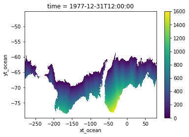
We will also apply a mask to our results, so we will only keep values for cells where SIC was greater or equal to 0.1.
[12]:
distances_t0.where(is_ice).plot()
[12]:
<matplotlib.collections.QuadMesh at 0x14c664500970>
Calculating results for other time steps
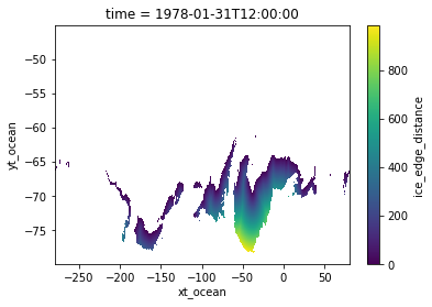
We can wrap this up into a function to calculate distances for a given timestep. This function returns the ice mask as a second value, so that we can make the plots in the same format as demonstrated so far.
[13]:
def ice_edge_distances(ice_ds):
    x, y = np.meshgrid(np.deg2rad(var_ice.xt_ocean.values),
                   np.deg2rad(var_ice.yt_ocean.values))
    grid_coords = np.vstack([y.flat, x.flat]).T

    is_ice = ice_ds >= 0.1
    cumulative_ice = is_ice.cumsum(dim='yt_ocean')
    ice_edge = (cumulative_ice == cumulative_ice.max('yt_ocean')) * is_ice

    ice_yt = ice_edge.yt_ocean[ice_edge.argmax(dim='yt_ocean')]
    ice_coords = np.vstack([ice_yt, ice_edge.xt_ocean]).T

    ball_tree = BallTree(np.deg2rad(ice_coords), metric='haversine')
    distances_radians, _ = ball_tree.query(grid_coords, return_distance=True)

    distances_km = distances_radians * 6371
    distances = xr.DataArray(
        data=distances_km.reshape(ice_ds.yt_ocean.size, -1),
        dims=['yt_ocean', 'xt_ocean'],
        coords={'yt_ocean': ice_ds.yt_ocean, 'xt_ocean': ice_ds.xt_ocean},
        name='ice_edge_distance'
    )

    return distances, is_ice
[14]:
distances_t1, mask = ice_edge_distances(var_ice.isel(time=1))

distances_t1.where(mask).plot()
[14]:
<matplotlib.collections.QuadMesh at 0x14c666b674c0>
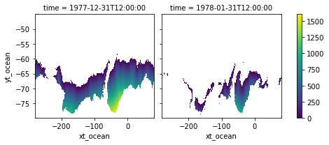
Stacking results into one data array
[15]:
dist_ice = xr.concat([distances_t0.where(is_ice), distances_t1.where(mask)], dim='time')
dist_ice
[15]:
<xarray.DataArray (time: 2, yt_ocean: 713, xt_ocean: 3600)>
dask.array<concatenate, shape=(2, 713, 3600), dtype=float64, chunksize=(1, 270, 360), chunktype=numpy.ndarray>
Coordinates:
  * yt_ocean  (yt_ocean) float64 -79.97 -79.93 -79.88 ... -45.18 -45.11 -45.04
  * xt_ocean  (xt_ocean) float64 -279.9 -279.8 -279.7 ... 79.75 79.85 79.95
  * time      (time) datetime64[ns] 1977-12-31T12:00:00 1978-01-31T12:00:00
[16]:
dist_ice.plot(col='time')
[16]:
<xarray.plot.facetgrid.FacetGrid at 0x14c666b0ac70>
You are done! You should be able to follow the same workflow to calculate distances to any line/point of your interest.