Comparing Model Resolution¶

Load and explore model solutions at a range of horizontal resolutions (1°, 0.25°, and 0.1°). We use snapshots of model output to explore how the velocity fields differ between the simulations. We also look at eddy kinetic energy, which highlights that coarser resolution simulations have less variability in their velocity fields.

[1]:

%config InlineBackend.figure_format='retina'

import cosima_cookbook as cc
import numpy as np
import xarray as xr
import cf_xarray as cfxr
import pint_xarray
from pint import application_registry as ureg

import matplotlib.pyplot as plt
import cartopy.crs as ccrs
import cartopy.feature as cft

Given that the high resolution simulations contain quite a lot of data, let’s fire up a Dask cluster to parallelise the computation.

[2]:

from dask.distributed import Client

client = Client()
client

[2]:

Client

Client-22d44f34-e284-11ee-8194-00000190fe80

Connection method: Cluster object	Cluster type: distributed.LocalCluster
Dashboard: /proxy/8787/status

Cluster Info

LocalCluster

b9057249

Dashboard: /proxy/8787/status	Workers: 4
Total threads: 12	Total memory: 46.00 GiB
Status: running	Using processes: True

Scheduler Info

Scheduler

Scheduler-05d5f966-f1de-492a-b6e1-95892f7a0a1f

Comm: tcp://127.0.0.1:34741	Workers: 4
Dashboard: /proxy/8787/status	Total threads: 12
Started: Just now	Total memory: 46.00 GiB

Workers

Worker: 0

Comm: tcp://127.0.0.1:36605	Total threads: 3
Dashboard: /proxy/45655/status	Memory: 11.50 GiB
Nanny: tcp://127.0.0.1:41537
Local directory: /jobfs/110881222.gadi-pbs/dask-scratch-space/worker-hs8j53s_

Worker: 1

Comm: tcp://127.0.0.1:32817	Total threads: 3
Dashboard: /proxy/39897/status	Memory: 11.50 GiB
Nanny: tcp://127.0.0.1:42353
Local directory: /jobfs/110881222.gadi-pbs/dask-scratch-space/worker-66fuqc_a

Worker: 2

Comm: tcp://127.0.0.1:45059	Total threads: 3
Dashboard: /proxy/32985/status	Memory: 11.50 GiB
Nanny: tcp://127.0.0.1:40749
Local directory: /jobfs/110881222.gadi-pbs/dask-scratch-space/worker-vv5yktv_

Worker: 3

Comm: tcp://127.0.0.1:45621	Total threads: 3
Dashboard: /proxy/41993/status	Memory: 11.50 GiB
Nanny: tcp://127.0.0.1:46821
Local directory: /jobfs/110881222.gadi-pbs/dask-scratch-space/worker-f46x5_b8

Now instantiate a database session.

[3]:

session = cc.database.create_session()

Pick three experiments to analyse. If you want to look at a list of all the experiments available, run the following snippet.

print(cc.querying.get_experiments(session)['experiment'].values)

[4]:

experiments = ['01deg_jra55v140_iaf_cycle4',
               '025deg_jra55_iaf_omip2_cycle6',
               '1deg_jra55_iaf_omip2_cycle6']

titles      = ['0.1° horizontal resolution',
               '0.25° horizontal resolution',
               '1° horizontal resolution']

For simplicity, here we load only 3 years of data. But you may load as much as you like! Also we only load one depth level, in particular the one prescribed with variable depth below.

[5]:

start_time = '1980-01-01'
end_time = '1982-12-31'
depth = 0

[6]:

sims = {}

for experiment in experiments:
    u = cc.querying.getvar(experiment, 'u', session,
                           frequency='1 monthly',
                           start_time=start_time,
                           end_time=end_time)

    v = cc.querying.getvar(experiment, 'v', session,
                           frequency='1 monthly',
                           start_time=start_time,
                           end_time=end_time)

    for coord in [u.xu_ocean, v.xu_ocean]:
        coord.attrs['standard_name'] = 'grid_longitude'
        coord.attrs['units'] = 'degree'

    for coord in [u.yu_ocean, v.yu_ocean]:
        coord.attrs['standard_name'] = 'grid_latitude'
        coord.attrs['units'] = 'degree'

    u = u.cf.sel(vertical=depth, method='nearest').sel(time=slice(start_time, end_time))
    v = v.cf.sel(vertical=depth, method='nearest').sel(time=slice(start_time, end_time))

    # attach units to datasets using pint
    u = u.pint.quantify()
    v = v.pint.quantify()

    speed = np.sqrt(u**2 + v**2) # since for MOM5 u and v live on the same grid

    eke = 1/2 * ((u - u.mean(dim='time'))**2 + (v - v.mean(dim='time'))**2)

    sims[experiment] = xr.merge([u, v, speed.rename('speed'), eke.rename('eke')])

/g/data/hh5/public/apps/miniconda3/envs/analysis3-24.01/lib/python3.10/site-packages/xarray/core/dataset.py:271: UserWarning: The specified chunks separate the stored chunks along dimension "xu_ocean" starting at index 120. This could degrade performance. Instead, consider rechunking after loading.
warnings.warn(
/g/data/hh5/public/apps/miniconda3/envs/analysis3-24.01/lib/python3.10/site-packages/xarray/core/dataset.py:271: UserWarning: The specified chunks separate the stored chunks along dimension "yu_ocean" starting at index 108. This could degrade performance. Instead, consider rechunking after loading.
warnings.warn(
/g/data/hh5/public/apps/miniconda3/envs/analysis3-24.01/lib/python3.10/site-packages/xarray/core/dataset.py:271: UserWarning: The specified chunks separate the stored chunks along dimension "xu_ocean" starting at index 120. This could degrade performance. Instead, consider rechunking after loading.
warnings.warn(
/g/data/hh5/public/apps/miniconda3/envs/analysis3-24.01/lib/python3.10/site-packages/xarray/core/dataset.py:271: UserWarning: The specified chunks separate the stored chunks along dimension "yu_ocean" starting at index 108. This could degrade performance. Instead, consider rechunking after loading.
warnings.warn(
/g/data/hh5/public/apps/miniconda3/envs/analysis3-24.01/lib/python3.10/site-packages/xarray/core/dataset.py:271: UserWarning: The specified chunks separate the stored chunks along dimension "xu_ocean" starting at index 120. This could degrade performance. Instead, consider rechunking after loading.
warnings.warn(
/g/data/hh5/public/apps/miniconda3/envs/analysis3-24.01/lib/python3.10/site-packages/xarray/core/dataset.py:271: UserWarning: The specified chunks separate the stored chunks along dimension "yu_ocean" starting at index 108. This could degrade performance. Instead, consider rechunking after loading.
warnings.warn(
/g/data/hh5/public/apps/miniconda3/envs/analysis3-24.01/lib/python3.10/site-packages/xarray/core/dataset.py:271: UserWarning: The specified chunks separate the stored chunks along dimension "xu_ocean" starting at index 120. This could degrade performance. Instead, consider rechunking after loading.
warnings.warn(
/g/data/hh5/public/apps/miniconda3/envs/analysis3-24.01/lib/python3.10/site-packages/xarray/core/dataset.py:271: UserWarning: The specified chunks separate the stored chunks along dimension "yu_ocean" starting at index 108. This could degrade performance. Instead, consider rechunking after loading.
warnings.warn(
/g/data/hh5/public/apps/miniconda3/envs/analysis3-24.01/lib/python3.10/site-packages/xarray/core/dataset.py:271: UserWarning: The specified chunks separate the stored chunks along dimension "time" starting at index 1. This could degrade performance. Instead, consider rechunking after loading.
warnings.warn(
/g/data/hh5/public/apps/miniconda3/envs/analysis3-24.01/lib/python3.10/site-packages/xarray/core/dataset.py:271: UserWarning: The specified chunks separate the stored chunks along dimension "time" starting at index 1. This could degrade performance. Instead, consider rechunking after loading.
warnings.warn(
/g/data/hh5/public/apps/miniconda3/envs/analysis3-24.01/lib/python3.10/site-packages/xarray/core/dataset.py:271: UserWarning: The specified chunks separate the stored chunks along dimension "time" starting at index 1. This could degrade performance. Instead, consider rechunking after loading.
warnings.warn(
/g/data/hh5/public/apps/miniconda3/envs/analysis3-24.01/lib/python3.10/site-packages/xarray/core/dataset.py:271: UserWarning: The specified chunks separate the stored chunks along dimension "time" starting at index 1. This could degrade performance. Instead, consider rechunking after loading.
warnings.warn(
/g/data/hh5/public/apps/miniconda3/envs/analysis3-24.01/lib/python3.10/site-packages/xarray/core/dataset.py:271: UserWarning: The specified chunks separate the stored chunks along dimension "xu_ocean" starting at index 180. This could degrade performance. Instead, consider rechunking after loading.
warnings.warn(
/g/data/hh5/public/apps/miniconda3/envs/analysis3-24.01/lib/python3.10/site-packages/xarray/core/dataset.py:271: UserWarning: The specified chunks separate the stored chunks along dimension "yu_ocean" starting at index 150. This could degrade performance. Instead, consider rechunking after loading.
warnings.warn(
/g/data/hh5/public/apps/miniconda3/envs/analysis3-24.01/lib/python3.10/site-packages/xarray/core/dataset.py:271: UserWarning: The specified chunks separate the stored chunks along dimension "xu_ocean" starting at index 180. This could degrade performance. Instead, consider rechunking after loading.
warnings.warn(
/g/data/hh5/public/apps/miniconda3/envs/analysis3-24.01/lib/python3.10/site-packages/xarray/core/dataset.py:271: UserWarning: The specified chunks separate the stored chunks along dimension "yu_ocean" starting at index 150. This could degrade performance. Instead, consider rechunking after loading.
warnings.warn(
/g/data/hh5/public/apps/miniconda3/envs/analysis3-24.01/lib/python3.10/site-packages/xarray/core/dataset.py:271: UserWarning: The specified chunks separate the stored chunks along dimension "xu_ocean" starting at index 180. This could degrade performance. Instead, consider rechunking after loading.
warnings.warn(
/g/data/hh5/public/apps/miniconda3/envs/analysis3-24.01/lib/python3.10/site-packages/xarray/core/dataset.py:271: UserWarning: The specified chunks separate the stored chunks along dimension "xu_ocean" starting at index 180. This could degrade performance. Instead, consider rechunking after loading.
warnings.warn(
/g/data/hh5/public/apps/miniconda3/envs/analysis3-24.01/lib/python3.10/site-packages/xarray/core/dataset.py:271: UserWarning: The specified chunks separate the stored chunks along dimension "yu_ocean" starting at index 150. This could degrade performance. Instead, consider rechunking after loading.
warnings.warn(
/g/data/hh5/public/apps/miniconda3/envs/analysis3-24.01/lib/python3.10/site-packages/xarray/core/dataset.py:271: UserWarning: The specified chunks separate the stored chunks along dimension "yu_ocean" starting at index 150. This could degrade performance. Instead, consider rechunking after loading.
warnings.warn(

Having loaded the data, let’s plot some output from each simulation and look at the differences. We select the final time of the loaded data to plot.

First we load the land that we’ll use in all plots.

[7]:

land_50m = cft.NaturalEarthFeature('physical', 'land', '50m',
                                   edgecolor='black', facecolor='lightgray', linewidth=0.5)

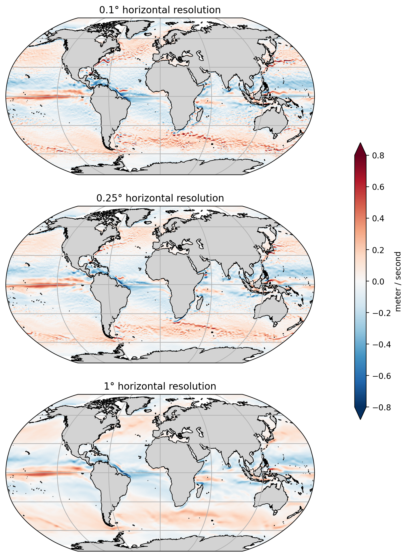
The following plots are snapshots of zonal velocity. All three simulations show roughly the same results, with westward and eastward flows occuring in approximately the same locations. However, the 0.1° and 0.25° simulations show mesoscale variability that is entirely lacking from the 1° simulation.

[8]:

fig, axes = plt.subplots(nrows = 3, figsize = (10, 12),
                         subplot_kw = {'projection': ccrs.Robinson()})

for counter, experiment in enumerate(experiments):
    ax = axes[counter]
    ax.coastlines(resolution='50m')
    ax.add_feature(land_50m)
    ax.gridlines(draw_labels=False)

    u_snapshot = sims[experiment].u.sel(time=sims[experiment].time[-1])

    p = u_snapshot.cf.plot(ax = ax,
                           x='grid_longitude',
                           y='grid_latitude',
                           transform=ccrs.PlateCarree(),
                           cmap='RdBu_r', vmin=-0.8, vmax=0.8,
                           add_colorbar=False)

    ax.set_title(titles[counter])

ax_cb = plt.axes([0.85, 0.3, 0.02, 0.4])
plt.colorbar(p, cax=ax_cb, extend='both', label=u_snapshot.pint.units);

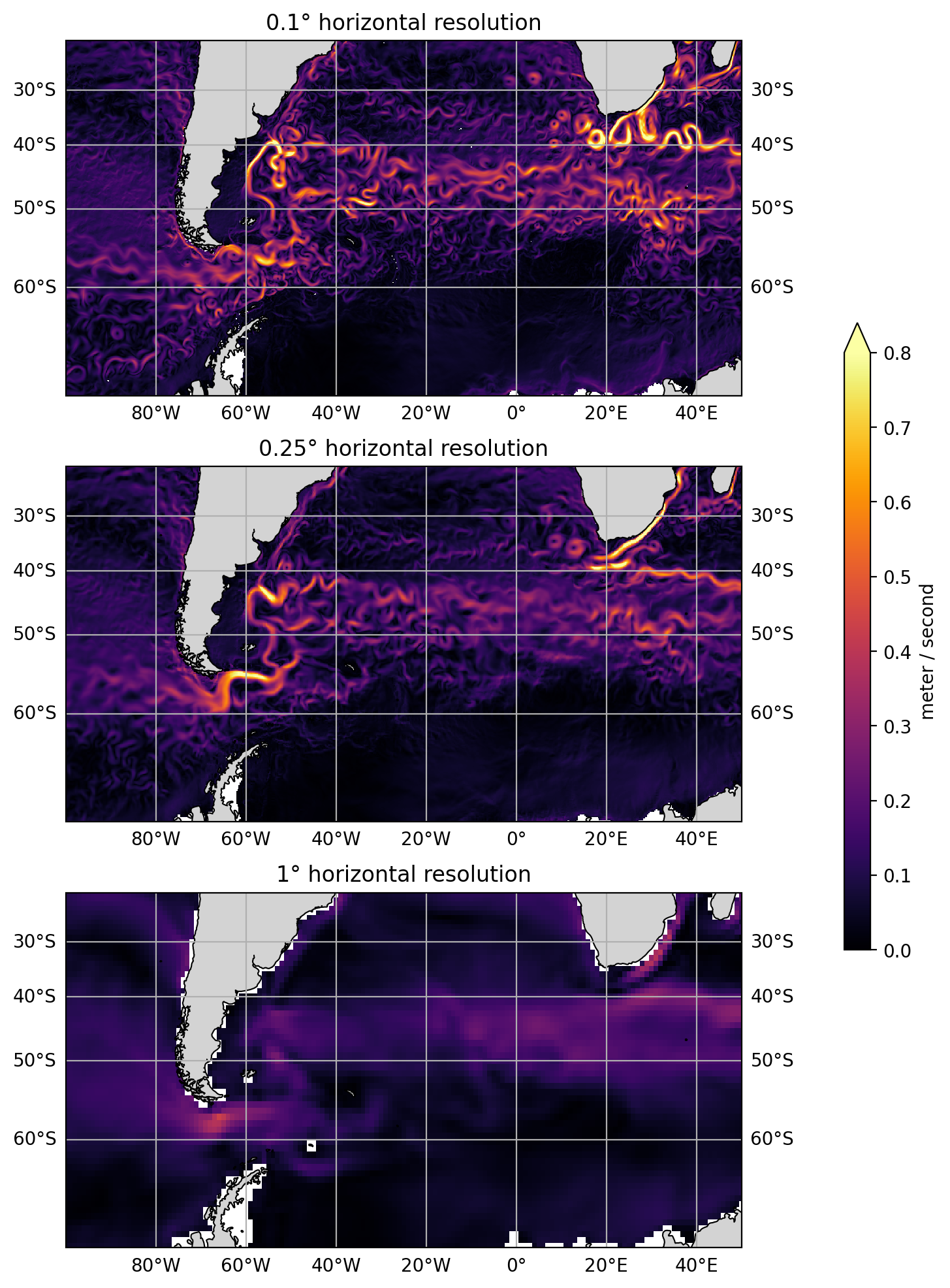
../_images/DocumentedExamples_Model_Resolution_Comparison_14_0.png

The mesoscale variability hinted at in the above global figures is more easily seen by zooming into a regional scale. The plots below show the Atlantic sector of the Southern Ocean, including the Agulhas Current, and Drake Passage. The figures below also show that higher horizontal resolution support much higher flow speeds.

[9]:

projection=ccrs.Mercator(central_longitude=0.0, min_latitude=-70.0, max_latitude=-20.0)

fig, axes = plt.subplots(nrows = 3, figsize = (10, 12),
                         subplot_kw = {'projection': projection})

for counter, experiment in enumerate(experiments):
    ax = axes[counter]
    ax.set_extent([-100, 50, -70, -20], crs=ccrs.PlateCarree())
    ax.coastlines(resolution='50m')
    ax.add_feature(land_50m)
    gl = ax.gridlines(draw_labels=True)
    gl.xlabels_top = False

    speed_snapshot = sims[experiment].speed.sel(time=sims[experiment].time[-1])

    p = speed_snapshot.cf.plot(ax=ax,
                               x='grid_longitude',
                               y='grid_latitude',
                               transform=ccrs.PlateCarree(),
                               cmap='inferno', vmin=0, vmax=0.8,
                               add_colorbar=False)

    ax.set_title(titles[counter])

ax_cb = plt.axes([0.85, 0.3, 0.02, 0.4])
plt.colorbar(p, cax=ax_cb, extend='max', label=speed_snapshot.pint.units);

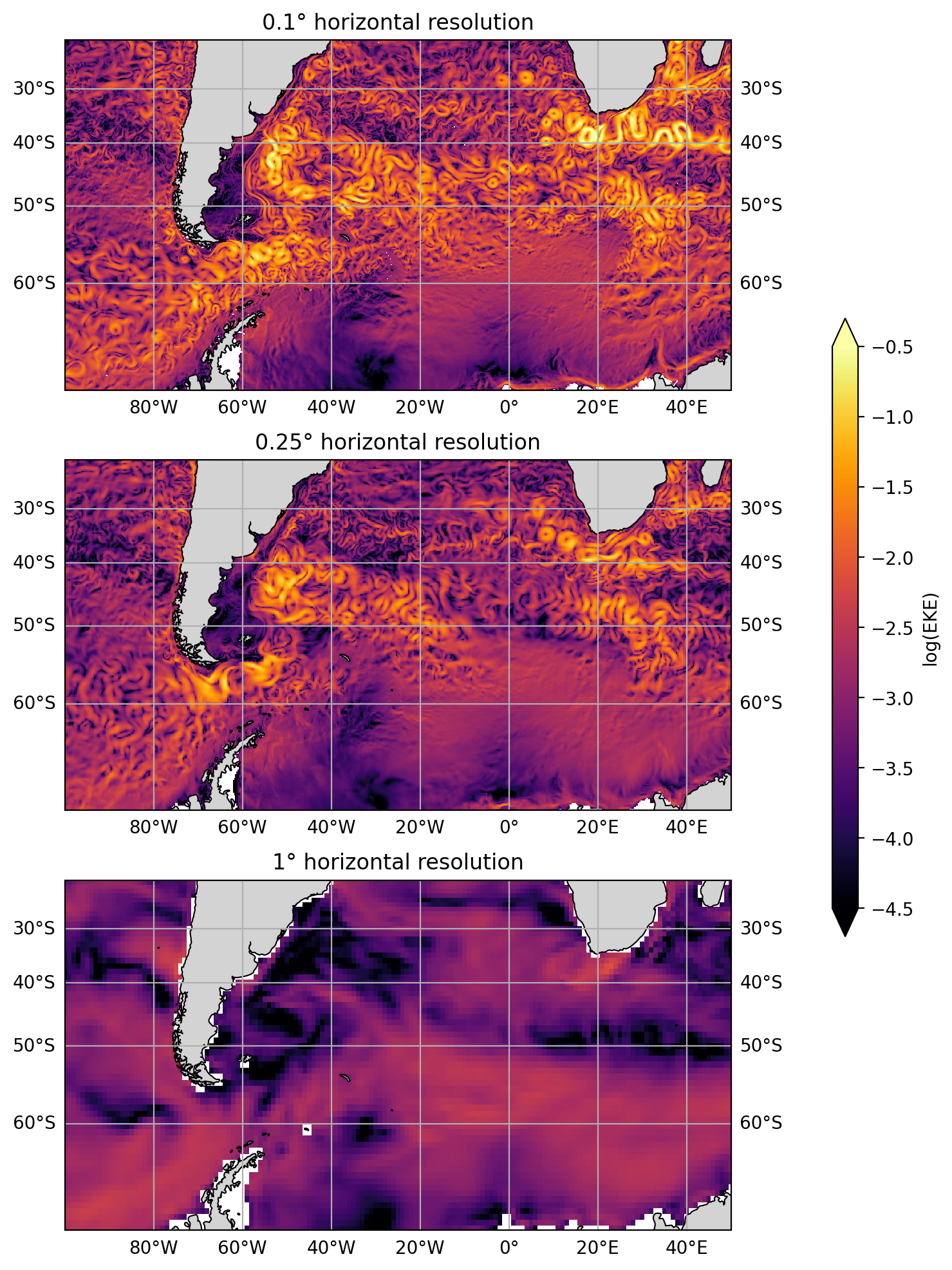
../_images/DocumentedExamples_Model_Resolution_Comparison_16_0.png

The higher resolution simulations exhibit much more variability in their velocity fields. This can be easily seen by looking at eddy kinetic energy, defined as

\[\text{EKE} = \frac1{2} \big[ (u - \overline{u})^{2} + (v-\overline{v})^{2} \big]\]

where overbar denotes a time average. Eddy kinetic energy picks out variability in the velocity fields. Again, we plot the final timestamp.

This plot takes quite some time to produce, since it requires averaging the entire time series of u and v for each simulation.

[10]:

projection=ccrs.Mercator(central_longitude=0.0, min_latitude=-70.0, max_latitude=-20.0)

fig, axes = plt.subplots(nrows = 3, figsize = (10, 12),
                         subplot_kw = {'projection': projection})

for counter, experiment in enumerate(experiments):
    ax = axes[counter]
    ax.set_extent([-100, 50, -70, -20], crs=ccrs.PlateCarree())
    ax.coastlines(resolution='50m')
    ax.add_feature(land_50m)
    gl = ax.gridlines(draw_labels=True)
    gl.xlabels_top = False

    eke_snapshot = sims[experiment].eke.sel(time=sims[experiment].time[-1])

    log10eke = np.log10(eke_snapshot.pint.dequantify()) # can't take logarithm of quantity with units

    p = log10eke.cf.plot(ax=ax,
                         x='grid_longitude',
                         y='grid_latitude',
                         transform=ccrs.PlateCarree(),
                         cmap='inferno', vmin=-4.5, vmax=-0.5,
                         add_colorbar=False)

    ax.set_title(titles[counter])

ax_cb = plt.axes([0.85, 0.3, 0.02, 0.4])
plt.colorbar(p, cax=ax_cb, extend='both', label='log(EKE)');

../_images/DocumentedExamples_Model_Resolution_Comparison_18_0.png