Meridional Heat Transport (MHT)
This notebook calculates the model MHT using three methods based on distinct MOM5 diagnostics. The methods are listed below along with the caveats that come with each one:
temp_yflux_adv_int_z(depth-integrated meridional heat transport due to resolved advection): This diagnostic is computed online and is therefore accurate. However, being an estimate of the advective meridional heat transport, it doesn’t contain any heat transport due to diffusive parameterizations in the model.net_sfc_heating(net surface heat flux): This method estimates the meridional heat transport and is approximate because of the steady state assumption. Ideally, frazil formation at higher latitudes should be added to the net surface heating variable, but we skip it here as the diagnostic is not available with this experiment.ty_trans,temp,dxanddzt(depth- and zonally-integrated product of meridional transport and temperature): This method is also approximate as it neglects contributions from time-varying correlations between meridional transport and temperature for frequencies faster than the output frequency of the diagnostics themselves.
Strictly speaking, the above methods compute reference-dependent heat flux at each latitude instead of meridional heat transport as there may be net meridional mass transports for which a unique heat transport cannot be defined. To compute a reference-temperature independent heat transport, the anomalous meridional mass transport needs to be subtracted from the total transport at each latitude (which is quite large in comparison to the anomaly).
To use this notebook, we need to ensure the above diagnostics are available in the model output. We can check if a variable is available using cc.querying.get_variables() function from the COSIMA cookbook.
NOTE: The third method is memory-intensive, so we recommend using at least 128 GB of memory. Alternatively, select a smaller temporal or spatial region of interest.
Currently this notebook calculates the total (all basins) MHT and it also includes comparisons to a few observational products. Basin-specific MHT can be calculated by defining relevant masks (see for e.g., https://github.com/COSIMA/cosima-recipes/blob/main/DocumentedExamples/Atlantic_IndoPacific_Basin_Overturning_Circulation.ipynb).
Loading relevant libraries
[1]:
import cosima_cookbook as cc
import numpy as np
import xarray as xr
import matplotlib.pyplot as plt
Start dask cluster.
[2]:
from dask.distributed import Client
client = Client()
client
[2]:
Client
Client-ef795084-7c78-11ee-b86e-000007e6fe80
| Connection method: Cluster object | Cluster type: distributed.LocalCluster |
| Dashboard: /proxy/8787/status |
Cluster Info
LocalCluster
0daab491
| Dashboard: /proxy/8787/status | Workers: 7 |
| Total threads: 28 | Total memory: 251.20 GiB |
| Status: running | Using processes: True |
Scheduler Info
Scheduler
Scheduler-b7b66cc7-2dc7-48fb-965d-8f662d6be263
| Comm: tcp://127.0.0.1:45899 | Workers: 7 |
| Dashboard: /proxy/8787/status | Total threads: 28 |
| Started: Just now | Total memory: 251.20 GiB |
Workers
Worker: 0
| Comm: tcp://127.0.0.1:43905 | Total threads: 4 |
| Dashboard: /proxy/36119/status | Memory: 35.89 GiB |
| Nanny: tcp://127.0.0.1:44101 | |
| Local directory: /jobfs/100038024.gadi-pbs/dask-scratch-space/worker-qv8h64x6 | |
Worker: 1
| Comm: tcp://127.0.0.1:40331 | Total threads: 4 |
| Dashboard: /proxy/46367/status | Memory: 35.89 GiB |
| Nanny: tcp://127.0.0.1:45083 | |
| Local directory: /jobfs/100038024.gadi-pbs/dask-scratch-space/worker-sml0_3p3 | |
Worker: 2
| Comm: tcp://127.0.0.1:45139 | Total threads: 4 |
| Dashboard: /proxy/40415/status | Memory: 35.89 GiB |
| Nanny: tcp://127.0.0.1:34305 | |
| Local directory: /jobfs/100038024.gadi-pbs/dask-scratch-space/worker-bqzhni39 | |
Worker: 3
| Comm: tcp://127.0.0.1:40233 | Total threads: 4 |
| Dashboard: /proxy/35697/status | Memory: 35.89 GiB |
| Nanny: tcp://127.0.0.1:41281 | |
| Local directory: /jobfs/100038024.gadi-pbs/dask-scratch-space/worker-8215tppk | |
Worker: 4
| Comm: tcp://127.0.0.1:34131 | Total threads: 4 |
| Dashboard: /proxy/38009/status | Memory: 35.89 GiB |
| Nanny: tcp://127.0.0.1:39981 | |
| Local directory: /jobfs/100038024.gadi-pbs/dask-scratch-space/worker-54fxpgaw | |
Worker: 5
| Comm: tcp://127.0.0.1:35343 | Total threads: 4 |
| Dashboard: /proxy/34417/status | Memory: 35.89 GiB |
| Nanny: tcp://127.0.0.1:44789 | |
| Local directory: /jobfs/100038024.gadi-pbs/dask-scratch-space/worker-o3nez__a | |
Worker: 6
| Comm: tcp://127.0.0.1:41379 | Total threads: 4 |
| Dashboard: /proxy/45607/status | Memory: 35.89 GiB |
| Nanny: tcp://127.0.0.1:41591 | |
| Local directory: /jobfs/100038024.gadi-pbs/dask-scratch-space/worker-t8ek86yr | |
Loading model data
We will use the COSIMA cookbook to search its database and load temp_yflux_adv_int_z to start our calculations. To do this we will need to do the following: 1. Start a COSIMA cookbook session 2. Define the model configuration of interest 3. Define the experiment of interest 4. Define the diagnostic (variable) of interest
NOTE: If you are in doubt about the models, experiments and diagnostics available in the database, check the Cookbook Tutorial for more information.
Start a cookbook session.
[3]:
session = cc.database.create_session()

#Define experiment of interest
experiment = '025deg_jra55v13_iaf_gmredi6'
We are now ready to query the database and load the data to start our analysis. We load temp_yflux_adv_int_z. For this example, we have chosen to use 6 years of output.
Method 1: using depth-integrated meridional heat transport due to resovled advection
[4]:
mht_method1 = cc.querying.getvar(experiment, 'temp_yflux_adv_int_z', session, n=3)
mht_method1
[4]:
<xarray.DataArray 'temp_yflux_adv_int_z' (time: 72, yu_ocean: 1080,
                                          xt_ocean: 1440)>
dask.array<concatenate, shape=(72, 1080, 1440), dtype=float32, chunksize=(1, 540, 720), chunktype=numpy.ndarray>
Coordinates:
  * yu_ocean  (yu_ocean) float64 -81.02 -80.92 -80.81 ... 89.79 89.89 90.0
  * time      (time) datetime64[ns] 2198-01-14T12:00:00 ... 2203-12-14T12:00:00
  * xt_ocean  (xt_ocean) float64 -279.9 -279.6 -279.4 ... 79.38 79.62 79.88
Attributes:
    long_name:      z-integral of cp*rho*dxt*v*temp
    units:          Watts
    valid_range:    [-1.e+18  1.e+18]
    cell_methods:   time: mean
    time_avg_info:  average_T1,average_T2,average_DT
    coordinates:    geolon_t geolat_c
ncfiles: ['/g/data/hh5/tmp/cosima/access-om2-025/025deg_jra55v13_i...Viewing the variable containing our data provides a number of key information, including: - Shape of dataset - In this case the data includes 72 time steps, 1080 steps along the y axis and 1440 along the x axis. - Name of coordinates - Our data includes time, yu_ocean (i.e., latitude), and xt_ocean (i.e., longitude). - Values included under each coordinate - We can see that time includes monthly values from 2198-01-14 to 2203-12-14. - Metadata - This information is
included under Attributes and it includes things like units.
Calculating mean and converting units
From the metadata, we can see that our dataset is in Watts (W), so we will convert them to petawatts (PW)
[5]:
# convert Watts -> PettaWatts
mht_method1 = (mht_method1 * 1e-15).assign_attrs(units='PettaWatts')
mht_method1
[5]:
<xarray.DataArray 'temp_yflux_adv_int_z' (time: 72, yu_ocean: 1080,
                                          xt_ocean: 1440)>
dask.array<mul, shape=(72, 1080, 1440), dtype=float32, chunksize=(1, 540, 720), chunktype=numpy.ndarray>
Coordinates:
  * yu_ocean  (yu_ocean) float64 -81.02 -80.92 -80.81 ... 89.79 89.89 90.0
  * time      (time) datetime64[ns] 2198-01-14T12:00:00 ... 2203-12-14T12:00:00
  * xt_ocean  (xt_ocean) float64 -279.9 -279.6 -279.4 ... 79.38 79.62 79.88
Attributes:
units: PettaWattsand then we compute the mean across time and sum over all longitudes.
[6]:
mht_method1 = mht_method1.mean('time').sum('xt_ocean')
mht_method1
[6]:
<xarray.DataArray 'temp_yflux_adv_int_z' (yu_ocean: 1080)>
dask.array<sum-aggregate, shape=(1080,), dtype=float32, chunksize=(540,), chunktype=numpy.ndarray>
Coordinates:
  * yu_ocean  (yu_ocean) float64 -81.02 -80.92 -80.81 ... 89.79 89.89 90.0
Method 2: using from the net surface heat flux (assuming steady state)
First, we load the surface heat flux and grid metrics:
[7]:
shflux = cc.querying.getvar(experiment, 'net_sfc_heating', session, n=3)
shflux_am = shflux.mean('time').load()

area = cc.querying.getvar(experiment, 'area_t', session, ncfile="ocean_grid.nc", n=1)
lat  = cc.querying.getvar(experiment, 'geolat_t', session, ncfile="ocean_grid.nc", n=1)
latv = cc.querying.getvar(experiment, 'yt_ocean', session, ncfile="ocean_grid.nc", n=1)
Now calculate Meridional Heat Flux (MHF):
Note: The following cell might take 1-2 min.
[8]:
%%time

mhf = xr.zeros_like(latv)

for i in range(len(latv)):
    inds = lat < latv[i]
    atmp = area.where(lat < latv[i])
    stmp = shflux_am.where(lat < latv[i])
    mhf[i] = np.sum(atmp * stmp)

mht_method2 = mhf + (mhf[0] - mhf[-1]) / 2
CPU times: user 1min 37s, sys: 12.8 s, total: 1min 49s
Wall time: 3min 26s
[9]:
# convert Watts -> PettaWatts
mht_method2 = (mht_method2 * 1e-15).assign_attrs(units='PettaWatts')
mht_method2
[9]:
<xarray.DataArray 'yt_ocean' (yt_ocean: 1080)>
array([ 0.11841208,  0.11841208,  0.11841208, ..., -0.11841084,
       -0.11841175, -0.11841208])
Coordinates:
  * yt_ocean  (yt_ocean) float64 -81.08 -80.97 -80.87 ... 89.74 89.84 89.95
Attributes:
units: PettaWattsMethod 3: Using 3D transport and potential temperature
This method computes the MHF using meridional transport (or alternatively, meridional velocities mapped on to the transport grid) and potential temperature diagnostics. For this method to work, the net transport across each latitude section must be zero. Then, the MHF can be understood as the product of northward (or southward) flow with the temperature difference between the northward and southward flow.
We choose an experiment which contains monthly data fields to capture monthly temporal correlations between meridional transport and temperature:
[10]:
experiment = '025deg_jra55_ryf9091_gadi'
We interpolate each variable on to \(x\)-center and \(y\)-face grid as we are estimating a tracer across a given latitude:
[11]:
V = cc.querying.getvar(experiment, 'ty_trans', session, frequency = '1 monthly', n = 3, use_cftime = True)

θ = cc.querying.getvar(experiment, 'temp', session, frequency = '1 monthly', n = 3, use_cftime = True)

# convert degK -> degC
θ = (θ - 273.15).assign_attrs(units='degrees C')

θ = θ.interp(yt_ocean = V.yu_ocean.values, method = "linear").rename({'yt_ocean': 'yu_ocean'})
- The meridional heat transport at a given latitude is then calculated using: :nbsphinx-math:`begin{equation}
MHF(y, t) = rho , C_p iint , v(x,y,z,t) , theta(x,y,z,t) , mathrm{d}x mathrm{d}z,
end{equation}` where we time-average the MHF in the end.
[12]:
%%time

Cp = 3992.10322329649  # heat capacity [J / (kg C)] used by MOM5

HT = (Cp * V * θ).sum('xt_ocean').sum('st_ocean').mean('time')

# convert Watts -> PettaWatts
mht_method3 = (HT * 1e-15).assign_attrs(units='PettaWatts').load()
mht_method3
CPU times: user 1min 25s, sys: 5.05 s, total: 1min 30s
Wall time: 2min 10s
[12]:
<xarray.DataArray (yu_ocean: 1080)>
array([ 0.0000000e+00,  0.0000000e+00,  0.0000000e+00, ...,
       -2.0530437e-04, -2.2442040e-05,  0.0000000e+00], dtype=float32)
Coordinates:
  * yu_ocean  (yu_ocean) float64 -81.02 -80.92 -80.81 ... 89.79 89.89 90.0
Attributes:
units: PettaWattsAdditional remarks on method 3
- Strictly speaking, the MHF calculated using the above formula contains a net meridional flow for each latitude, which makes the MHF dependent on the temperature scale. We can ensure zero net transport across a given latitude by subtracting mean flow (\(v_m(y,t)\)) across that latitude: :nbsphinx-math:`begin{equation}
v_m(y,t) = frac{iint v(x,y,z,t) , mathrm{d}x mathrm{d}z}{iint , mathrm{d}x mathrm{d}z},
- end{equation}` where \(v(x,y,z,t)\) is the meridional velocity at a given latitude. From this, the no-mean velocity (\(v_{nm} (x,y,z,t)\)) is given by: :nbsphinx-math:`begin{equation}
v_{nm} (x,y,z,t) = v(x,y,z,t) - v_m(y,t).
end{equation}`
- The no-mean velocity (not estimated numerically in this notebook) could then used to evaluate the MHF using: :nbsphinx-math:`begin{equation}
MHF(y,t) = rho C_piint v_{nm}(x,y,z,t), theta(x,y,z,t) , mathrm{d}x mathrm{d}z,
end{equation}` where we time-average the MHF in the end.
Comparison between model output and observations
Before producing our figure, we compare the model output with observations to check the model accuracy. These observations are derived using various methods, in particular using surface flux observations and method 2 (which assumes a steady state).
Read ERBE Period Ocean and Atmospheric Heat Transport
Observations are also available on gadi, here we show how to load them to our notebook.
[13]:
#Path to the file containing observations
filename = '/g/data3/hh5/tmp/cosima/observations/original/MHT/obs_vq_am_estimates.txt'

#Creating empty variables to store our observations
erbe_mht = []
erbe_lat = []

#Opening data and saving it to empty variables above
with open(filename) as f:
    #Open each line from rows 1 to 96
    for line in f.readlines()[1:96]:
        #Separating each line to extract data
        line = line.strip()
        sline = line.split()
        #Extracting latitude and MHT and saving to empty variables
        erbe_lat.append(float(sline[0]))
        erbe_mht.append(float(sline[3]))

#Checking MHT variables
erbe_mht
[13]:
[7.82256e-05,
 -0.00548183,
 -0.00534277,
 -0.00778958,
 -0.0153764,
 -0.0189109,
 -0.0172473,
 -0.0321044,
 -0.0647783,
 -0.104008,
 -0.129806,
 -0.202605,
 -0.297446,
 -0.374377,
 -0.424618,
 -0.464923,
 -0.508466,
 -0.544651,
 -0.56517,
 -0.575634,
 -0.563567,
 -0.51931,
 -0.45106,
 -0.377069,
 -0.310393,
 -0.271679,
 -0.279999,
 -0.329881,
 -0.39744,
 -0.464742,
 -0.515384,
 -0.565431,
 -0.620221,
 -0.678495,
 -0.736833,
 -0.790937,
 -0.843637,
 -0.90752,
 -0.984516,
 -1.05272,
 -1.0956,
 -1.10212,
 -1.05218,
 -0.93882,
 -0.761357,
 -0.502307,
 -0.155427,
 0.253559,
 0.666604,
 1.00846,
 1.25254,
 1.42962,
 1.57235,
 1.69269,
 1.78862,
 1.84355,
 1.85095,
 1.82898,
 1.79722,
 1.76105,
 1.71365,
 1.65596,
 1.59826,
 1.53441,
 1.45553,
 1.34517,
 1.20096,
 1.03473,
 0.856831,
 0.704894,
 0.62273,
 0.602973,
 0.60382,
 0.602437,
 0.599438,
 0.588678,
 0.573292,
 0.5557,
 0.518399,
 0.46073,
 0.40554,
 0.361088,
 0.328643,
 0.303888,
 0.271855,
 0.232879,
 0.18562,
 0.146825,
 0.110927,
 0.0737569,
 0.0460509,
 0.0254577,
 0.0100299,
 0.00272631,
 0.000137086]
Read NCEP and ECMWF Oceanic and Atmospheric Transport Products
These datasets are available at https://climatedataguide.ucar.edu/climate-data. We use a climatological mean of surface fluxes or vertically integrated total energy divergence for oceanic and atmospheric transports respectively for the period between February 1985 - April 1989.
[14]:
#Path to the file containing observations
filename = '/g/data3/hh5/tmp/cosima/observations/original/MHT/ANNUAL_TRANSPORTS_1985_1989.ascii'

#Creating empty variables to store our observations
ncep_g_mht = []
ecwmf_g_mht = []
ncep_g_err = []
ecwmf_g_err = []
ncep_a_mht = []
ecwmf_a_mht = []
ncep_a_err = []
ecwmf_a_err = []
ncep_p_mht = []
ecwmf_p_mht = []
ncep_p_err = []
ecwmf_p_err = []
ncep_i_mht = []
ecwmf_i_mht = []
ncep_i_err = []
ecwmf_i_err = []
ncep_ip_mht = []
ecwmf_ip_mht = []
ncep_ip_err = []
ecwmf_ip_err = []
o_lat = []

#Opening data and saving it to empty variables above
with open(filename) as f:
#Open each line in file (ignoring the first row)
    for line in f.readlines()[1:]:
        #Separating each line to extract data
        line = line.strip()
        sline = line.split()
        #Extracting values and saving to correct variable defined above
        o_lat.append(float(sline[0])*0.01)  # T42 latitudes (north to south)
        ncep_g_mht.append(float(sline[4])*0.01) # Residual Ocean Transport - NCEP
        ecwmf_g_mht.append(float(sline[5])*0.01)# Residual Ocean Transport - ECWMF
        ncep_a_mht.append(float(sline[7])*0.01)# Atlantic Ocean Basin Transport - NCEP
        ncep_p_mht.append(float(sline[8])*0.01)# Pacific Ocean Basin Transport - NCEP
        ncep_i_mht.append(float(sline[9])*0.01)# Indian Ocean Basin Transport - NCEP
        ncep_g_err.append(float(sline[10])*0.01)# Error Bars for NCEP Total Transports
        ncep_a_err.append(float(sline[11])*0.01)# Error Bars for NCEP Atlantic Transports
        ncep_p_err.append(float(sline[12])*0.01)# Error Bars for NCEP Pacific Transports
        ncep_i_err.append(float(sline[13])*0.01)# Error Bars for NCEP Indian Transports
        ecwmf_a_mht.append(float(sline[15])*0.01)# Atlantic Ocean Basin Transport - ECWMF
        ecwmf_p_mht.append(float(sline[16])*0.01)# Pacific Ocean Basin Transport - ECWMF
        ecwmf_i_mht.append(float(sline[17])*0.01)# Indian Ocean Basin Transport - ECWMF
        ecwmf_g_err.append(float(sline[18])*0.01)# Error Bars for ECWMF Total Transports
        ecwmf_a_err.append(float(sline[19])*0.01)# Error Bars for NCEP Atlantic Transports
        ecwmf_p_err.append(float(sline[20])*0.01)# Error Bars for NCEP Pacific Transports
        ecwmf_i_err.append(float(sline[21])*0.01)# Error Bars for NCEP Indian Transports

#Calculating MHT
ncep_ip_mht  = [a+b for a, b in zip(ncep_p_mht,ncep_i_mht)]
ecwmf_ip_mht = [a+b for a, b in zip(ecwmf_p_mht,ecwmf_i_mht)]
ncep_ip_err  = [max(a, b) for a, b in zip(ncep_p_err, ncep_i_err)]
ecwmf_ip_err = [max(a, b) for a, b in zip(ecwmf_p_err, ecwmf_i_err)]
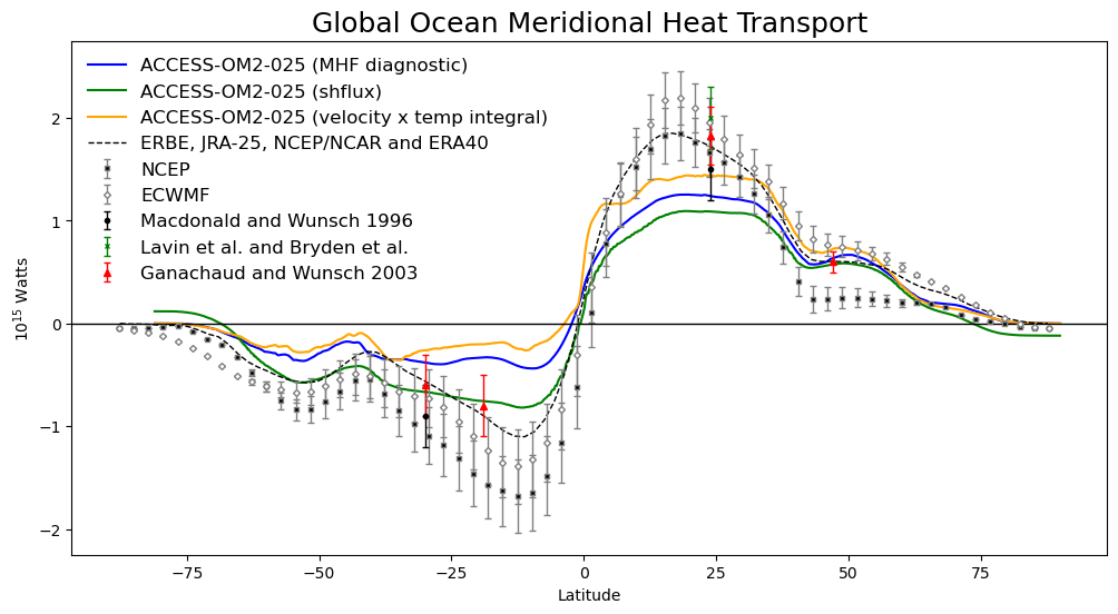
Plotting model outputs against observations
We plot the global meridional heat transport as calculated from model outputs (blue line) and observations.
[15]:
fig = plt.figure(figsize=(12, 6))
ax = fig.add_subplot(1, 1, 1)

#Plotting MHT from model outputs
mht_method1.plot(ax = ax, color = "blue", label = "ACCESS-OM2-025 (MHF diagnostic)")
mht_method2.plot(ax = ax, color = "green", label = "ACCESS-OM2-025 (shflux)")
mht_method3.plot(ax = ax, color = 'orange', label = 'ACCESS-OM2-025 (velocity x temp integral)')

#Adding observations and error bars for observations
ax.plot(erbe_lat, erbe_mht, 'k--', linewidth=1, label="ERBE, JRA-25, NCEP/NCAR and ERA40")
plt.errorbar(o_lat[::-1], ncep_g_mht[::-1], yerr=ncep_g_err[::-1], c='gray', fmt='s',
             markerfacecolor='k', markersize=3, capsize=2, linewidth=1, label="NCEP")
plt.errorbar(o_lat[::-1], ecwmf_g_mht[::-1], yerr=ecwmf_g_err[::-1], c='gray', fmt='D',
             markerfacecolor='white', markersize=3, capsize=2, linewidth=1, label="ECWMF")
plt.errorbar( 24,  1.5,  yerr=0.3,  fmt='o', c='black', markersize=3, capsize=2, linewidth=1,
             label="Macdonald and Wunsch 1996")
plt.errorbar(-30, -0.9,  yerr=0.3,  fmt='o', c='black', markersize=3, capsize=2, linewidth=1)
plt.errorbar( 24,  2.0,  yerr=0.3,  fmt='x', c='green', markersize=3, capsize=2, linewidth=1,
             label="Lavin et al. and Bryden et al.")
plt.errorbar( 24,  1.83, yerr=0.28, fmt='^', c='red',   markersize=4, capsize=2, linewidth=1,
             label="Ganachaud and Wunsch 2003")
plt.errorbar(-30, -0.6,  yerr=0.3,  fmt='^', c='red',   markersize=4, capsize=2, linewidth=1)
plt.errorbar(-19, -0.8,  yerr=0.3,  fmt='^', c='red',   markersize=4, capsize=2, linewidth=1)
plt.errorbar( 47,  0.6,  yerr=0.1,  fmt='^', c='red',   markersize=4, capsize=2, linewidth=1)

#Adding legend
plt.legend(frameon=False, fontsize=12)
plt.axhline(y=0, linewidth=1, color='black')

#Defining plot limits along the y axis
plt.ylim(-2.25, 2.75)

#Adding titles for figure and axes
plt.title('Global Ocean Meridional Heat Transport', fontsize=18)
plt.xlabel('Latitude')
plt.ylabel('$10^{15}$ Watts');