Meridional Overturning Circulation
This recipe shows an example of calculating the zonally-averaged global meridional overturning circulation using output from MOM6. We compute the overturning circulation both in density–latitude and depth–latitude space. We also plot separate basin-averaged overturning streamfunctions.
Requirements: The conda/analysis3-25.06 (or later) module on ARE. We recommend an ARE session with more than 14 cores to make these computations. Ideally, use a whole Gadi compute node from normalbw, i.e., 28 cores.
‼️ ⚠️ 🚨 Caveats 🚨 ⚠️ ‼️
The computations presented in this recipe suffer from two issues in the Arctic ocean region, north of 65\(^\circ\)N:
The overturning metrics in this notebook do not use correct zonal averaging in the tripole region, north of 65\(^\circ\)N! See https://cosima-recipes.readthedocs.io/en/latest/02-Easy-Recipes/True_Zonal_Mean.html for a recipe explainig how to properly average quantities in the zonal direction when the north of 65\(^\circ\)N.
The notion of vector quantities is distorted north of 65\(^\circ\)N, because north of 65\(^\circ\)N the grid cells’ local
x- andy- directions do not align with lines of constant latitude and longitude. Thereforevno longer gives the true meridional transport north of 65ᵒN. To correctly compute the overturning north of 65\(^\circ\)N, we would need to rotate the volume transports in the localx- andy-directions to obtain the corresponding transports in the zonal and meridional direction. For that reason, all computations done in this notebook are wrong north of 65\(^\circ\)N, and we only show latitudes south of 65\(^\circ\)N in the plots. See https://github.com/COSIMA/cosima-recipes/issues/510 for more details.
Information needed to adapt to MOM5:
Diagnostics needed:
ty_trans_rho: meridional transport binned online intorho2layers. This is on the same grid asvmo, i.e. the centre of the northern tracer cell’s face.pot_rho_2: potential density referenced to 2000 metres needed to remapping the overturning to depth coordinates.
Notes
For low-resolution MOM5-based runs that include mesoscale eddy flux parameterisations, we need to explicitly include the volume transport from the Gent-McWilliams eddy parameterisation (ty_trans_rho_gm). This transport is already cumulatively summed in the vertical (see section 32.3.1 of the MOM5 manual), so it needs to be added after the cumulative sum of ty_trans_rho when calculating the overturning streamfuncton
psi (see this example). For MOM6 we don’t need to worry about this, because it is already included in vmo. Similarly, all resolutions in ACCESS-OM2 MOM5 have parameterised submesoscale meridional transport (ty_trans_submeso) which is already cumulatively summed in the vertical and not included in ty_trans_rho. However, it tends
to be relatively unimportant for the deep circulation, which is where we are primarily interested, so we are probably can safely ignore it. Again, for MOM6, this is conveniently already included in the vmo output.
MOM6 Recipe:
[1]:
import numpy as np
import xarray as xr

from dask.distributed import Client

import matplotlib.pyplot as plt
import cmocean as cm

import intake
cat = intake.cat.access_nri
[2]:
client = Client(threads_per_worker = 1)
client
[2]:
Client
Client-8efad3ff-7508-11f1-a825-00000399fe80
| Connection method: Cluster object | Cluster type: distributed.LocalCluster |
| Dashboard: /proxy/8787/status |
Cluster Info
LocalCluster
7a1bb684
| Dashboard: /proxy/8787/status | Workers: 28 |
| Total threads: 28 | Total memory: 128.00 GiB |
| Status: running | Using processes: True |
Scheduler Info
Scheduler
Scheduler-717d1414-d397-4483-9dca-d57f6a0cf163
| Comm: tcp://127.0.0.1:36357 | Workers: 0 |
| Dashboard: /proxy/8787/status | Total threads: 0 |
| Started: Just now | Total memory: 0 B |
Workers
Worker: 0
| Comm: tcp://127.0.0.1:38741 | Total threads: 1 |
| Dashboard: /proxy/39351/status | Memory: 4.57 GiB |
| Nanny: tcp://127.0.0.1:40023 | |
| Local directory: /jobfs/172781226.gadi-pbs/dask-scratch-space/worker-d2n96v4t | |
Worker: 1
| Comm: tcp://127.0.0.1:46787 | Total threads: 1 |
| Dashboard: /proxy/37763/status | Memory: 4.57 GiB |
| Nanny: tcp://127.0.0.1:40417 | |
| Local directory: /jobfs/172781226.gadi-pbs/dask-scratch-space/worker-3jnhedt_ | |
Worker: 2
| Comm: tcp://127.0.0.1:34007 | Total threads: 1 |
| Dashboard: /proxy/41561/status | Memory: 4.57 GiB |
| Nanny: tcp://127.0.0.1:44359 | |
| Local directory: /jobfs/172781226.gadi-pbs/dask-scratch-space/worker-xnpkiqdv | |
Worker: 3
| Comm: tcp://127.0.0.1:45397 | Total threads: 1 |
| Dashboard: /proxy/38059/status | Memory: 4.57 GiB |
| Nanny: tcp://127.0.0.1:37351 | |
| Local directory: /jobfs/172781226.gadi-pbs/dask-scratch-space/worker-dn3sq748 | |
Worker: 4
| Comm: tcp://127.0.0.1:41547 | Total threads: 1 |
| Dashboard: /proxy/40583/status | Memory: 4.57 GiB |
| Nanny: tcp://127.0.0.1:40095 | |
| Local directory: /jobfs/172781226.gadi-pbs/dask-scratch-space/worker-aunrkaq_ | |
Worker: 5
| Comm: tcp://127.0.0.1:38443 | Total threads: 1 |
| Dashboard: /proxy/36495/status | Memory: 4.57 GiB |
| Nanny: tcp://127.0.0.1:39011 | |
| Local directory: /jobfs/172781226.gadi-pbs/dask-scratch-space/worker-_b46vbj3 | |
Worker: 6
| Comm: tcp://127.0.0.1:34719 | Total threads: 1 |
| Dashboard: /proxy/37595/status | Memory: 4.57 GiB |
| Nanny: tcp://127.0.0.1:40001 | |
| Local directory: /jobfs/172781226.gadi-pbs/dask-scratch-space/worker-elwjz3p7 | |
Worker: 7
| Comm: tcp://127.0.0.1:44823 | Total threads: 1 |
| Dashboard: /proxy/44961/status | Memory: 4.57 GiB |
| Nanny: tcp://127.0.0.1:36319 | |
| Local directory: /jobfs/172781226.gadi-pbs/dask-scratch-space/worker-w3v8da8n | |
Worker: 8
| Comm: tcp://127.0.0.1:44611 | Total threads: 1 |
| Dashboard: /proxy/40687/status | Memory: 4.57 GiB |
| Nanny: tcp://127.0.0.1:35937 | |
| Local directory: /jobfs/172781226.gadi-pbs/dask-scratch-space/worker-xg02b4ww | |
Worker: 9
| Comm: tcp://127.0.0.1:38647 | Total threads: 1 |
| Dashboard: /proxy/45171/status | Memory: 4.57 GiB |
| Nanny: tcp://127.0.0.1:33447 | |
| Local directory: /jobfs/172781226.gadi-pbs/dask-scratch-space/worker-2sxvzzrd | |
Worker: 10
| Comm: tcp://127.0.0.1:36733 | Total threads: 1 |
| Dashboard: /proxy/33705/status | Memory: 4.57 GiB |
| Nanny: tcp://127.0.0.1:44523 | |
| Local directory: /jobfs/172781226.gadi-pbs/dask-scratch-space/worker-ggxpka01 | |
Worker: 11
| Comm: tcp://127.0.0.1:34223 | Total threads: 1 |
| Dashboard: /proxy/44467/status | Memory: 4.57 GiB |
| Nanny: tcp://127.0.0.1:40257 | |
| Local directory: /jobfs/172781226.gadi-pbs/dask-scratch-space/worker-9rwga45y | |
Worker: 12
| Comm: tcp://127.0.0.1:42855 | Total threads: 1 |
| Dashboard: /proxy/37727/status | Memory: 4.57 GiB |
| Nanny: tcp://127.0.0.1:39247 | |
| Local directory: /jobfs/172781226.gadi-pbs/dask-scratch-space/worker-bacry3hu | |
Worker: 13
| Comm: tcp://127.0.0.1:35053 | Total threads: 1 |
| Dashboard: /proxy/46727/status | Memory: 4.57 GiB |
| Nanny: tcp://127.0.0.1:33395 | |
| Local directory: /jobfs/172781226.gadi-pbs/dask-scratch-space/worker-0_dtjfjh | |
Worker: 14
| Comm: tcp://127.0.0.1:35963 | Total threads: 1 |
| Dashboard: /proxy/42733/status | Memory: 4.57 GiB |
| Nanny: tcp://127.0.0.1:37407 | |
| Local directory: /jobfs/172781226.gadi-pbs/dask-scratch-space/worker-7w9ljdjp | |
Worker: 15
| Comm: tcp://127.0.0.1:33687 | Total threads: 1 |
| Dashboard: /proxy/36659/status | Memory: 4.57 GiB |
| Nanny: tcp://127.0.0.1:46267 | |
| Local directory: /jobfs/172781226.gadi-pbs/dask-scratch-space/worker-xtc9su0v | |
Worker: 16
| Comm: tcp://127.0.0.1:36481 | Total threads: 1 |
| Dashboard: /proxy/36499/status | Memory: 4.57 GiB |
| Nanny: tcp://127.0.0.1:33643 | |
| Local directory: /jobfs/172781226.gadi-pbs/dask-scratch-space/worker-qnh57912 | |
Worker: 17
| Comm: tcp://127.0.0.1:45227 | Total threads: 1 |
| Dashboard: /proxy/44607/status | Memory: 4.57 GiB |
| Nanny: tcp://127.0.0.1:36075 | |
| Local directory: /jobfs/172781226.gadi-pbs/dask-scratch-space/worker-jnb351q9 | |
Worker: 18
| Comm: tcp://127.0.0.1:39827 | Total threads: 1 |
| Dashboard: /proxy/46563/status | Memory: 4.57 GiB |
| Nanny: tcp://127.0.0.1:32817 | |
| Local directory: /jobfs/172781226.gadi-pbs/dask-scratch-space/worker-542vyzfp | |
Worker: 19
| Comm: tcp://127.0.0.1:34517 | Total threads: 1 |
| Dashboard: /proxy/34371/status | Memory: 4.57 GiB |
| Nanny: tcp://127.0.0.1:43301 | |
| Local directory: /jobfs/172781226.gadi-pbs/dask-scratch-space/worker-xjkwifsc | |
Worker: 20
| Comm: tcp://127.0.0.1:38667 | Total threads: 1 |
| Dashboard: /proxy/41933/status | Memory: 4.57 GiB |
| Nanny: tcp://127.0.0.1:39051 | |
| Local directory: /jobfs/172781226.gadi-pbs/dask-scratch-space/worker-xyg1kna5 | |
Worker: 21
| Comm: tcp://127.0.0.1:39525 | Total threads: 1 |
| Dashboard: /proxy/36693/status | Memory: 4.57 GiB |
| Nanny: tcp://127.0.0.1:43977 | |
| Local directory: /jobfs/172781226.gadi-pbs/dask-scratch-space/worker-lgmtk116 | |
Worker: 22
| Comm: tcp://127.0.0.1:34573 | Total threads: 1 |
| Dashboard: /proxy/38357/status | Memory: 4.57 GiB |
| Nanny: tcp://127.0.0.1:43271 | |
| Local directory: /jobfs/172781226.gadi-pbs/dask-scratch-space/worker-449t16s3 | |
Worker: 23
| Comm: tcp://127.0.0.1:34957 | Total threads: 1 |
| Dashboard: /proxy/32959/status | Memory: 4.57 GiB |
| Nanny: tcp://127.0.0.1:46681 | |
| Local directory: /jobfs/172781226.gadi-pbs/dask-scratch-space/worker-22zgrvor | |
Worker: 24
| Comm: tcp://127.0.0.1:37213 | Total threads: 1 |
| Dashboard: /proxy/43273/status | Memory: 4.57 GiB |
| Nanny: tcp://127.0.0.1:40235 | |
| Local directory: /jobfs/172781226.gadi-pbs/dask-scratch-space/worker-cldiaddp | |
Worker: 25
| Comm: tcp://127.0.0.1:42267 | Total threads: 1 |
| Dashboard: /proxy/35171/status | Memory: 4.57 GiB |
| Nanny: tcp://127.0.0.1:43633 | |
| Local directory: /jobfs/172781226.gadi-pbs/dask-scratch-space/worker-yv5u37t_ | |
Worker: 26
| Comm: tcp://127.0.0.1:40009 | Total threads: 1 |
| Dashboard: /proxy/45847/status | Memory: 4.57 GiB |
| Nanny: tcp://127.0.0.1:37509 | |
| Local directory: /jobfs/172781226.gadi-pbs/dask-scratch-space/worker-jtstt_29 | |
Worker: 27
| Comm: tcp://127.0.0.1:42781 | Total threads: 1 |
| Dashboard: /proxy/44773/status | Memory: 4.57 GiB |
| Nanny: tcp://127.0.0.1:42117 | |
| Local directory: /jobfs/172781226.gadi-pbs/dask-scratch-space/worker-vaymp2qu | |
For this example, we are using 1 year of a 25 km ACCESS-OM3 IAF simulation. If you want to increase the resolution or integrate over a longer time you might need a bigger ARE session.
Note: We are using this experiment because it is currently to only global MOM6 output with the necessary output.
First we load up vmo and sum in the zonal direction.
Most ACCESS-OM2 and MOM6 simulations output mass transport (with units of kg/s), so we convert to volume transport, i.e., to Sverdrup (Sv = 10\(^6\) m\(^3\)/s).
[3]:
experiment = "MC_25km_jra_iaf+wombatlite-test3v2-00532b88"
start_time = "1990-01-01"
end_time = "1990-12-31"

# Because this is only a test simulation, not permanent data, it is not in the main ACCESS-NRI
# intake catalog, so we need to give instructions for where to find the relevant intake catalog:
OM3_datastore = intake.open_esm_datastore(
    "/g/data/ol01/outputs/access-om3-25km/MC_25km_jra_iaf+wombatlite-test3v2-00532b88/datastore.json",
    columns_with_iterables=[
            "variable",
            "variable_long_name",
            "variable_standard_name",
            "variable_cell_methods",
            "variable_units",
    ] # This is important
)

# We need to specify "file_id" here, because there is "vmo" saved both on depth and density coordinates.
# ".*" here is wildcard to ensure that the filenames contain "rho2_l", i.e., the density coordinate name.
df = OM3_datastore.search(variable="vmo", frequency="1mon", file_id=".*rho2_l.*")
vmo = df.to_dask(xarray_open_kwargs={"decode_timedelta": True}).vmo
vmo = vmo.sel(time=slice(start_time, end_time))

# convert mass transport -> volume transport and then convert units -> Sv
rho0 = 1035 # kg/m^3, average seawater density
psi = (vmo / rho0) / 1e6
psi.attrs["units"] = "Sv"

# sum in longitude:
psi_sum_lon = psi.sum("xh")

# Cumulatively sum the transport in the vertical, time average and load.
# Note that we want to sum from the bottom up, but .cumsum sums from the top down,
# which is why we substract the sum in the second term here:
psi_avg = psi_sum_lon.cumsum("rho2_l") - psi_sum_lon.sum("rho2_l")
psi_avg = psi_avg.mean("time")
psi_avg = psi_avg.load()
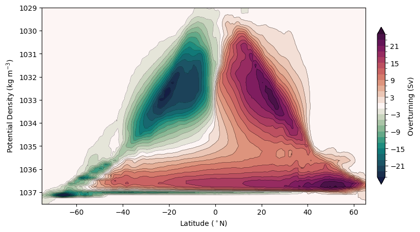
Plotting in density coordinates
Now we are ready to plot. We usually plot the streamfunction over a reduced range of density levels to highlight the deep ocean contribution.
[4]:
def levels_and_colorbarticks(max_value):
    """ Return the levels and the colorbarticks for the streamfunction plot.
    It may seem complicated but the truth is we just want to avoid the 0 contour
    so that the plot looks soothing to the eye.
    Note this function can result in mismatched contour levels and ticks if you
    change max_psi below to be an even number. """

    levels = np.hstack((np.arange(-max_value, 0, 2), np.flip(-np.arange(-max_value, 0, 2))))
    cbarticks = np.hstack((np.flip(-np.arange(3, max_value, 6)), np.arange(3, max_value, 6)))

    return levels, cbarticks
[5]:
plt.figure(figsize=(10, 5))

# Best if this is an odd number - otherwise levels and cbarticks may be mismatched:
max_psi = 25 # Sv

levels, cbarticks = levels_and_colorbarticks(max_psi)

psi_avg.plot.contourf(levels=levels,
                      cmap=cm.cm.curl,
                      extend='both',
                      cbar_kwargs={
                          'shrink': 0.8,
                          'label': 'Overturning (Sv)',
                          'ticks': cbarticks,
                          'pad': 0.03,
                      })

psi_avg.plot.contour(levels=levels,
                     colors='k',
                     linewidths=0.25)

plt.gca().invert_yaxis()

plt.ylim((1037.5, 1010))
plt.ylabel('Potential Density (kg m$^{-3}$)')
plt.xlabel('Latitude ($^\circ$N)')
# Limit to 65ᵒN, because calculations are wrong for region north of 65ᵒN, see https://github.com/COSIMA/cosima-recipes/issues/510
plt.xlim([-75, 65]);
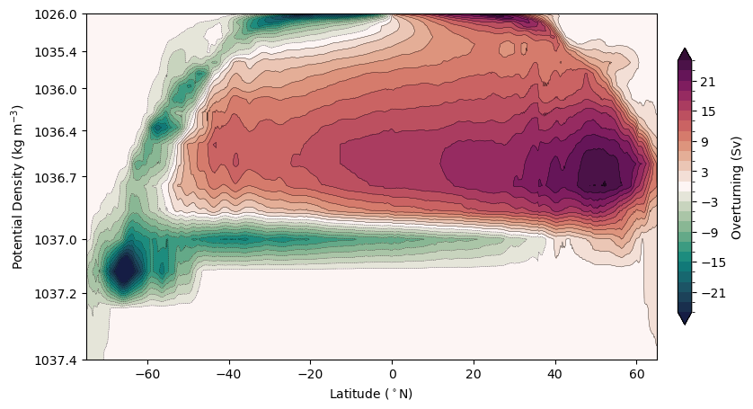
Alternatively, you may want to stretch the y-axis to minimise the visual impact of the surface circulation, while showing the full-depth ocean.
[6]:
# This code stretches the upper and lower density ranges separately,
# so the really low densities don't disappear in the stretching.

# Parameters to tune:
rho_break = 1030      # density where the stretching changes
low_fraction = 0.25     # fraction of plot height used for lighter densities
dense_stretch = 8       # strength of zoom in dense waters

# Limit density range before plotting:
rho_max = 1037.25
psi_avg_limited = psi_avg.sel(rho2_l=slice(None, rho_max))

rho = psi_avg_limited.rho2_l
rho_min = float(rho.min())

# Piecewise stretched density coordinate:
rho_stretched = xr.where(
    rho <= rho_break,
    low_fraction * (rho - rho_min) / (rho_break - rho_min),
    low_fraction + (1 - low_fraction) *
    ((rho - rho_break) / (rho_max - rho_break))**dense_stretch
)

psi_avg_plot = psi_avg_limited.assign_coords(rho2_l=rho_stretched)
[7]:
# Plot overturning with the stretched coordinate:
fig, ax = plt.subplots(1, 1, figsize=(10, 5))

max_psi = 25  # Sv
levels, cbarticks = levels_and_colorbarticks(max_psi)

psi_avg_plot.plot.contourf(
    ax=ax,
    levels=levels,
    cmap=cm.cm.curl,
    extend='both',
    cbar_kwargs={
        'shrink': 0.8,
        'label': 'Overturning (Sv)',
        'ticks': cbarticks,
        'pad': 0.03
    }
)

psi_avg_plot.plot.contour(
    ax=ax,
    levels=levels,
    colors='k',
    linewidths=0.25
)

yticks = np.array([
    1010, 1020, 1030, 1035.8, 1036.4, 1036.8, 1037.0, 1037.2
])

yticks_stretched = np.where(
    yticks <= rho_break,
    low_fraction * (yticks - rho_min) / (rho_break - rho_min),
    low_fraction + (1 - low_fraction) *
    ((yticks - rho_break) / (rho_max - rho_break))**dense_stretch
)

ax.set_yticks(yticks_stretched)
ax.set_yticklabels(yticks)
ax.set_ylim(1, 0)
ax.set_ylabel('Potential Density (kg m$^{-3}$)')
ax.set_xlabel('Latitude ($^\circ$N)')
ax.set_xlim([-75, 65])  # calculations are wrong north of 65°N

# Draw a horizontal line where the stretching changes:
ax.axhline(low_fraction, color='k', linewidth=1.0, linestyle='--');
Plotting in depth coordinates
Sometimes it’s nice to see what this looks like in depth space, because it’s a bit more intuitive. This requires remapping from density to depth space.
Unfortunately it seems not possible to do this density to depth conversion in the MC_25km_jra_iaf+wombatlite-test3v2-00532b88 experiment, because the zonal average of rhopot2 is non-monotonic nearly everywhere. If you want an example of this that works in MOM5, there is one here: https://github.com/COSIMA/cosima-recipes/blob/v0.1.7/03-Advanced-Recipes/Overturning_Circulation.ipynb
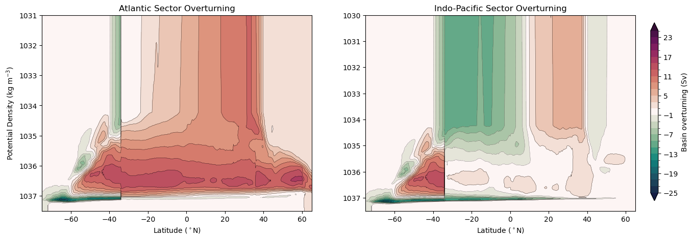
Atlantic and Indo-Pacific basin components of the Meridional Overturning Circulation
Here, we compute the zonally averaged meridional overturning streamfunction in density space in a similar fashion to the above, except that we partition the overturning circulation into the Atlantic and Indo-Pacific Basins. Strong North Atlantic deep water circulation in the Atlantic can sometimes obscure Antarctic Bottom Water circulation in the IndoPacific in global zonally-averaged calculations, something we can minimise by the masking procedure below.
Compute times were calculated using 28 cpus and 124 GB memory Jupyter Lab on gadi, using conda environment analysis3-25.06.
Create Masks for the Atlantic and IndoPacific Basins
Here we want to create two masks; one that masks for the Southern Ocean south of 33\(^\circ\)S (around the bottom of Africa) and the Atlantic Ocean, and one that masks for the Southern Ocean south of 33\(^\circ\)S and the Indian plus Pacific Oceans.
A bit of fiddling is a little unavoidable here but the procedure below should be compatible with 0.25\(^\circ\) or 1\(^\circ\) grid data so you don’t have to repeat the whole process.
To start with, load a single density layer of the overturning variable that we want to mask, because this is on the correct grid. We will make our mask from this.
[8]:
vmo = OM3_datastore.search(variable="vmo", frequency="1mon", file_id=".*rho2_l.*")
vmo = vmo.to_dask(xarray_open_kwargs={"use_cftime": True}).isel(time=0).isel(rho2_l=0).vmo
Now, make a land_mask. This is just a dataarray with 1’s where you have ocean and 0’s where you have land. We are going to work with this mask to delineate the different ocean basins.
[9]:
land_mask = ~vmo.isnull()
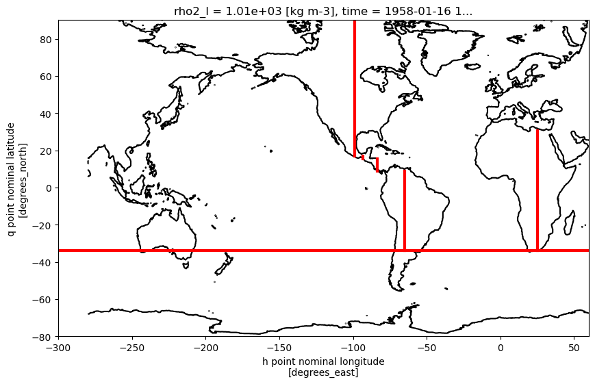
Now, let’s draw in a set of meridians that lie within land masses separating the Atlantic basin from the Indo-Pacific basins, to show where our mask is going to go. We will also have a line to delineate the southern boundary.
Note that the problems with this mask are:
It is not perfect at the Panama Canal;
The Great Australian Bight is not counted in the Southern Ocean;
The calculation is done on tracer points, but streamfunction is actually found on the northern edge of the tracer grid; and
We have ignored the tripole, so zonal averages north of 65°N are not so meaningful. That is of no consequence for the Pacific, but more relevant for the Atlantic/Arctic sector.
These are all pretty minor issues for a global quantity like the overturning, but users should feel free to improve this if they like.
[10]:
fig = plt.figure(2, (10, 6))
ax = plt.subplot()

land_mask.plot.contour(levels=[0.5], colors='k')

ax.plot([-300, 60], [-34,-34], 'r', linewidth = 3)
ax.plot([-65, -65], [-34, 9], 'r', linewidth = 3)
ax.plot([-83.7, -83.7], [9, 15.5], 'r', linewidth = 3)
ax.plot([-93.3, -93.3], [15.5, 17], 'r', linewidth = 3)
ax.plot([-99, -99], [17, 90], 'r', linewidth = 3)
ax.plot([25, 25], [-34,30.5], 'r', linewidth = 3)
ax.plot([79, 79], [30.5, 90], 'r', linewidth = 3)

ax.set_xlim([-300, 60])
ax.set_ylim([-80, 90]);
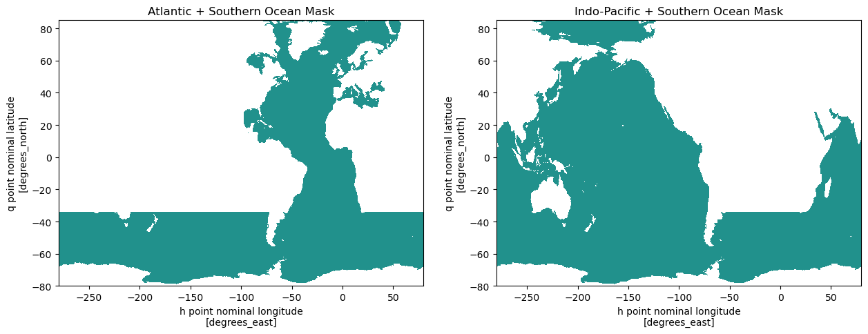
Now, let’s make our masks along these dividing lines. Note that we include the Southern Ocean in both the Atlantic and the Indo-Pacific masks.
[11]:
## create masks out of the above chunks
south_map = (land_mask.where(land_mask.yq < -34)).fillna(0)
indo_map1 = (land_mask.where(land_mask.yq < 9).where(land_mask.yq > -34).where(land_mask.xh > -280).where(land_mask.xh < -65)).fillna(0)
indo_map2 = (land_mask.where(land_mask.yq < 15).where(land_mask.yq > 9).where(land_mask.xh > -280).where(land_mask.xh < -83.7)).fillna(0)
indo_map3 = (land_mask.where(land_mask.yq < 17).where(land_mask.yq > 15).where(land_mask.xh > -280).where(land_mask.xh < -93.3)).fillna(0)
indo_map4 = (land_mask.where(land_mask.yq < 85).where(land_mask.yq > 17).where(land_mask.xh > -280).where(land_mask.xh < -99)).fillna(0)
indo_map5 = (land_mask.where(land_mask.yq < 30.5).where(land_mask.yq > -34).where(land_mask.xh > 25).where(land_mask.xh < 80)).fillna(0)

indo_sector_map = indo_map1 + indo_map2 + indo_map3 + indo_map4 + indo_map5 + south_map
indo_sector_mask = indo_sector_map.where(indo_sector_map>0)

atlantic_sector_map = (indo_sector_mask * 0).fillna(1) * land_mask
atlantic_sector_map = atlantic_sector_map + south_map
atlantic_sector_mask = atlantic_sector_map.where(atlantic_sector_map > 0)
[12]:
fig, ax = plt.subplots(1, 2, figsize=(15, 5))

atlantic_sector_mask.plot(ax=ax[0], add_colorbar=False)
ax[0].set_ylim([-80, 85])
ax[0].set_title('Atlantic + Southern Ocean Mask')

indo_sector_mask.plot(ax=ax[1], add_colorbar=False)
ax[1].set_ylim([-80, 85])
ax[1].set_title('Indo-Pacific + Southern Ocean Mask');
Mask psi by Basin and Compute Basin-Specific MOC
We use the psi from before, apply the mask and compute the basin-specific streamfunction in a similar manner as we did above.
[13]:
# Atlantic-MOC
Atlantic_psi = (psi * atlantic_sector_mask).sum("xh")
Atlantic_psi = Atlantic_psi.cumsum("rho2_l") - Atlantic_psi.sum("rho2_l")
Atlantic_psi = Atlantic_psi.mean("time")
Atlantic_psi = Atlantic_psi.load()

# Indo-Pacific MOC
IndoPacific_psi = (psi * indo_sector_mask).sum("xh")
IndoPacific_psi = IndoPacific_psi.cumsum("rho2_l") - IndoPacific_psi.sum("rho2_l")
IndoPacific_psi = IndoPacific_psi.mean("time")
IndoPacific_psi = IndoPacific_psi.load()
Plotting
Now plot the output.
[14]:
fig, ax = plt.subplots(1, 2, figsize=(15, 5))

# Best if this is an odd number - otherwise levels and cbarticks may be mismatched:
max_psi = 25 # Sv

levels, cbarticks = levels_and_colorbarticks(max_psi)

# Atlantic MOC
Atlantic_psi.plot.contourf(ax=ax[0],
                           levels=levels,
                           cmap=cm.cm.curl,
                           extend='both',
                           add_colorbar=False)
Atlantic_psi.plot.contour(ax=ax[0],
                          levels=levels,
                          colors='k',
                          linewidths=0.25)
ax[0].invert_yaxis()
ax[0].set_ylim((1037.5, 1031))
ax[0].set_ylabel('Potential Density (kg m$^{-3}$)')
ax[0].set_xlabel('Latitude ($^\circ$N)')
ax[0].set_title('Atlantic Sector Overturning')

# Limit to 65ᵒN, because calculations are wrong for region north of 65ᵒN, see https://github.com/COSIMA/cosima-recipes/issues/510
ax[0].set_xlim([-75, 65])


# Indo-Pacific MOC
h = IndoPacific_psi.plot.contourf(ax=ax[1],
                                  levels=levels,
                                  cmap=cm.cm.curl,
                                  extend='both',
                                  add_colorbar=False)
IndoPacific_psi.plot.contour(ax=ax[1],
                             levels=levels,
                             colors='k',
                             linewidths=0.25)
ax[1].invert_yaxis()
ax[1].set_ylim((1037.5, 1030))
ax[1].set_ylabel('')
ax[1].set_xlabel('Latitude ($^\circ$N)')
ax[1].set_title('Indo-Pacific Sector Overturning')

# Limit to 65ᵒN, because calculations are wrong for region north of 65ᵒN, see https://github.com/COSIMA/cosima-recipes/issues/510
ax[1].set_xlim([-75, 65])

# Plot a colorbar
cax = plt.axes([0.92, 0.15, 0.01, 0.7])
cb = plt.colorbar(h, cax=cax, orientation='vertical')
cb.ax.set_ylabel('Basin overturning (Sv)');
[ ]: