This notebook calculates neutral density (\(\gamma\)) in MOM6 using the algorithm developed by Jackett and McDougall 1997.
Before using neutral density, be aware that this is a calculation that uses as a reference a climatology from the World Atlas, Levitus 1980. Therefore, it shouldn’t be used for simulations or datasets with climates/ocean states different to the 1980s (i.e. future projection simulations).
Note that temperature in MOM5 is given as a conservative temperature in Kelvin, so you will need to (a) convert to Celsius and (b) go straight into calculating insitu temperature. All these diagnostics are in the t-cells, with xt_ocean and yt_ocean as longitude and latitude.
Let’s load the data - we will need temperature, salinity and depth - and select our region of interest. This recipe the pygamma function that only takes in 2D fields, so there is a parallelisation involved in calculating it for a time-varying 3D field. Be mindful of not making your region too big.
pygamma_n takes in in-situ temperature and absolute salinity, so we will use gsw to convert. This involves calculating pressure as well! And annoyingly to go from MOM6’s potential temperature to in situ temperature, we have to calculate conservative temperature as an intermediate step.
[9]:
# Get values of coordinatesdepth_coordinate=potential_temperature['z_l']longitudes=potential_temperature['xh']latitudes=potential_temperature['yh']# Calculate pressure to use as a coordinatepressure_coordinate=gsw.p_from_z(-depth_coordinate,latitudes)# Calculate absolute salinityabsolute_salinity=gsw.SA_from_SP(practical_salinity,pressure_coordinate,longitudes,latitudes).rename('SA')# Calculate conservative temperature (needed to calculate in situ temperatures)conservative_temperature=gsw.CT_from_pt(absolute_salinity,potential_temperature)# Calculate insitu temperatureinsitu_temperature=gsw.t_from_CT(absolute_salinity,conservative_temperature,pressure_coordinate).rename('t')
[10]:
insitu_temperature=insitu_temperature.load()
The pygamma_n function to calculate neutral densities takes 2D fields (cross sections with depth and lat/lon). So for our time-varying, 3D fields we are going to need to “iterate” twice, once through time and once through longitudes. We will define a function that calculates \(\gamma\) for a certain time step and longitude, and then use the Parallel function from joblib to calculate each cross section in parallel.
[11]:
defneutral_density(t,s,time_index,longitude_index):""" Calculates neutral density (gamma) for a given longitude and time of in-situ temperature and practical salinity datasets. """pressure=gsw.p_from_z(-t['z_l'],t['yh'])gamma,dg_lo,dg_hi=pygamma_n.gamma_n(s.isel(time=time_index,xh=longitude_index).transpose(),t.isel(time=time_index,xh=longitude_index).transpose(),pressure.transpose(),(t['xh'][longitude_index].item()*(t['yh']*0+1)),(t['yh']))gamma=gamma.Treturngamma
Now that we have our function, we need to make a list of arguments we want to feed it (every combination possible of time and longitude indexes):
[12]:
# Create a list of pairs that have a unique time, lon indexNt=len(insitu_temperature['time'])Nx=len(insitu_temperature['xh'])args_list=[[i,j]foriinrange(Nt)forjinrange(Nx)]
The cell below uses Parallel to run the neutral density function for each cross section in parallel, where the results are arranged as a list:
[13]:
# Run the neutral_density function in parallelresults=Parallel(n_jobs=-1)(delayed(neutral_density)(insitu_temperature,practical_salinity,arg1,arg2)forarg1,arg2inargs_list)
We need to reshape that list onto a DataArray with appropriate dimensions:
[14]:
# Reshape into the original dataset shapegamma=np.nan*np.zeros(np.shape(insitu_temperature))foridx,resultinenumerate(results):i,j=divmod(idx,Nx)gamma[i,:,:,j]=result
Convert gamma into a dataarray with dimensions and attributes.
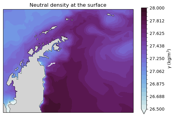
Let’s create a land mask and do a map of the time mean neutral density at the surface:
[17]:
# Create a land maskland_mask=xr.where(np.isnan(depth),1,np.nan)
[18]:
fig=plt.figure(figsize=(15,15))projection=ccrs.Mercator(central_longitude=-55)axs=fig.add_subplot(121,projection=projection)# Set the regionaxs.set_extent([-70,-40,-70,-60],crs=ccrs.PlateCarree())# Add model land maskland_mask.plot.contourf(ax=axs,colors='lightgrey',transform=ccrs.PlateCarree(),add_colorbar=False,zorder=2)# Add model coastlineland_mask.fillna(0).plot.contour(ax=axs,colors='k',levels=[0,1],transform=ccrs.PlateCarree(),add_colorbar=False,linewidths=0.5,zorder=3)# Plot time-mean neutral density at the surfacegamma.mean('time').isel(z_l=0).plot.pcolormesh(ax=axs,cmap=cmocean.cm.dense,transform=ccrs.PlateCarree(),vmin=26.5,vmax=28,levels=25,cbar_kwargs={'label':'$\\gamma$ (kg/m$^{3}$)','shrink':.3})axs.set_title('Neutral density at the surface');
[19]:
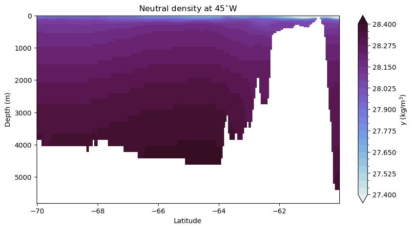
fig,axs=plt.subplots(figsize=(10,5))gamma.mean('time').sel(xh=-45,method='nearest').plot.pcolormesh(ax=axs,cmap=cmocean.cm.dense,vmin=27.4,vmax=28.4,levels=25,cbar_kwargs={'label':'$\\gamma$ (kg/m$^{3}$)'})axs.invert_yaxis()axs.set_ylabel('Depth (m)')axs.set_xlabel('Latitude')axs.set_title('Neutral density at 45$^{\circ}$W');