Calculate the true zonal mean of a scalar quantity regardless of the horizontal mesh.
Specifically, we calculate the volume weighted mean along all grid cells whose centres fall within finite latitude intervals rather than the arithmetic mean of cells along the model’s curvilinear grid. The method presented can also be used to re-grid models onto the same latitudinal grid and the general principles can be used to define any multidimensional sum or average using the xhistogram package.
Requirements: Select the conda/analysis3-25.09 (or later) kernel. This code should work for just about any MOM5 configuration since all we are grabbing is temeprature and standard grid information. We can swap temperature with any other scalar variable. We can also, in principle, swap latitude with another scalar.
Local directory: /jobfs/157096073.gadi-pbs/dask-scratch-space/worker-vdlo6oum
Open ACCESS-NRI’s default catalog:
[3]:
catalog=intake.cat.access_nri
Choose the experiment and the variable we want to average. This example uses temperature but you can choose any scalar, 3D variable. The variables dzt and area_t are also required so we can only use experiments that save those:
Intake dataframe catalog with 9 source(s) across 19 rows:
model
description
realm
frequency
variable
name
025deg_jra55_iaf_era5comparison
{ACCESS-OM2}
{0.25 degree ACCESS-OM2 global model configuration with JRA55-do v1.5.0\ninterannual forcing (1980-2019)}
{ocean}
{fx, 1mon}
{area_t, temp}
025deg_jra55_iaf_omip2_cycle1
{ACCESS-OM2}
{Cycle 1/6 of 0.25 degree ACCESS-OM2 physics-only global configuration with JRA55-do v1.4 OMIP2 interannual forcing (1958-2019)}
{ocean}
{fx, 1mon}
{area_t, temp}
025deg_jra55_iaf_omip2_cycle2
{ACCESS-OM2}
{Cycle 1/6 of 0.25 degree ACCESS-OM2 physics-only global configuration with JRA55-do v1.4 OMIP2 interannual forcing (1958-2019)}
{ocean}
{fx, 1mon}
{area_t, temp}
025deg_jra55_iaf_omip2_cycle3
{ACCESS-OM2}
{Cycle 3/6 of 0.25 degree ACCESS-OM2 physics-only global configuration with JRA55-do v1.4 OMIP2 interannual forcing (1958-2019)}
{ocean}
{fx, 1mon}
{area_t, temp}
025deg_jra55_iaf_omip2_cycle4
{ACCESS-OM2}
{Cycle 4/6 of 0.25 degree ACCESS-OM2 physics-only global configuration with JRA55-do v1.4 OMIP2 interannual forcing (1958-2019)}
{ocean}
{fx, 1mon}
{area_t, temp}
025deg_jra55_iaf_omip2_cycle5
{ACCESS-OM2}
{Cycle 5/6 of 0.25 degree ACCESS-OM2 physics-only global configuration with JRA55-do v1.4 OMIP2 interannual forcing (1958-2019)}
{ocean}
{fx, 1mon}
{area_t, temp}
025deg_jra55_iaf_omip2_cycle6
{ACCESS-OM2}
{Cycle 6/6 of 0.25 degree ACCESS-OM2 physics-only global configuration with JRA55-do v1.4 OMIP2 interannual forcing (1958-2019)}
{ocean}
{fx, 1mon}
{area_t, temp}
025deg_jra55_ryf9091_gadi
{ACCESS-OM2}
{0.25 degree ACCESS-OM2 physics-only global configuration with JRA55-do v1.3 RYF9091 repeat year forcing (May 1990 to Apr 1991)}
{ocean}
{fx, 1yr, 1mon}
{area_t, temp, dzt}
025deg_jra55_ryf_era5comparison
{ACCESS-OM2}
{0.25 degree ACCESS-OM2 global model configuration with JRA55-do v1.4.0\nRYF9091 repeat year forcing (May 1990 to Apr 1991)}
{ocean}
{fx, 1mon}
{area_t, temp, dzt}
[5]:
experiment='025deg_jra55_ryf9091_gadi'# any experiment that includes the required variablesvariable='temp'# any scalar variable for which volume-weighted average makes sensexarray_open_kwargs=dict(use_cftime=True,chunks={"time":-1},decode_timedelta=False)
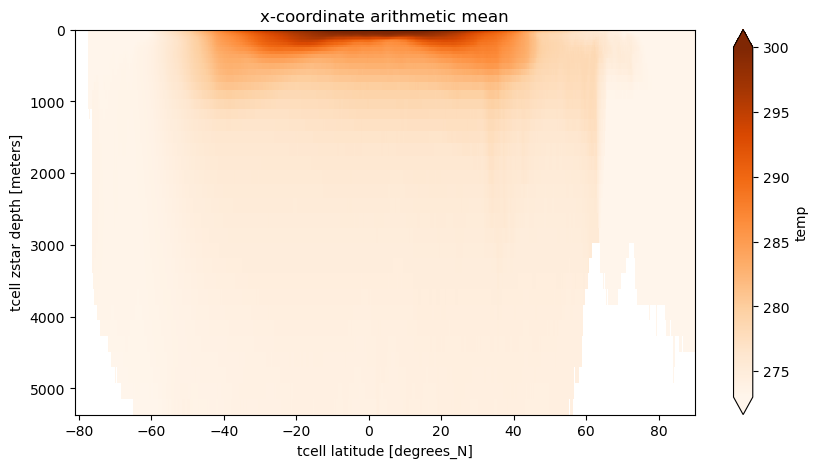
First we show the standard approach, which is to take the arithmetic mean of all grid cells along the quasi-longitudinal coordinate. For MOM5’s tri-polar grid this approach is in principle “okay” for the southern hemisphere, where grid cell areas are constant at fixed latitude. It doesn’t though, take into account partial cells.
The xarray’s method .mean(dim='dimension') applies numpy.mean() across that dimension. This is simply the arithmetic mean.
For some scalar \(T\) the arithmetic mean, e.g., across dimension i, is given by
where \(i\), \(j\) and \(k\) are the indicies in the \(x\), \(y\) and \(z\) directions respectively of the curvilinear grid and \(I\) is the number of indicies along the \(x\) axis.
CPU times: user 1.57 s, sys: 214 ms, total: 1.78 s
Wall time: 1.87 s
The main issue with this average is that the ‘latitude’ coordinate may be meaningless near the north pole, particularly when comparing to observational analyses or other models which can have either a regular grid or a different curvilinear grid. Even different versions of MOM might have different grids!
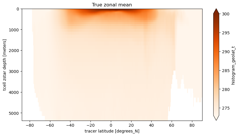
Let us consider what the true zonal average looks like. That is consider a set of latitude ‘edges’ \(\{\phi'_{1/2},\phi'_{1+1/2},...,\phi'_{\ell-1/2},\phi'_{\ell+1/2},...,\phi'_{L+1/2}\}\) between which we want to compute an average of \(T\) at \(\{\phi'_{1},\phi'_{2},...,\phi'_{\ell},...,\phi'_{L}\}\) such that
where \(\delta_{i,j} = 1\) if \(\phi'_{\ell-1/2}<\phi_{i,j}\leq \phi'_{\ell+1/2}\) and \(\delta_{i,j} = 0\) elsewhere, \(\Delta Z\) is the grid cell vertical thickness and \(\Delta \mathrm{Area}\) is the grid cell horizontal area.
For our purposes we will use the edges of the models xt_ocean coordinate to define \(\phi'_{\ell+1/2}\) so the number of ‘bins’ \(L\) will be the same as the length of the quasi-latitude coordinate (\(J\)).
Fortunately, as you can see below, the two sums are weighted histograms (one for \(T\) times volume and the other for just volume) and these can be rapidly computed using xhistogram.
First let’s load the scalar variable (latitude) we want to use as our coordinate then define the bin edges.
[8]:
coord='geolat_t'# can be any scalar (2D, 3D, eulerian, lagrangian etc)var_search=cat_subset.search(variable=coord,frequency='fx')variable_as_coord=var_search.to_dask(xarray_open_kwargs=dict(use_cftime=True))[coord]variable_as_coord
Now we want to define the coordinate bins as the latitude edges of the t-cells, adding the first edge (0) at latitude -90:
[9]:
# Define the coordinate bins as the latitude edges of the T-cellsvar_search=cat_subset.search(variable='geolat_c',frequency='fx')yu_ocean=var_search.to_dask(xarray_open_kwargs=dict(use_cftime=True))['yu_ocean']# make numpy array (using .values) and add 1st edge at -90bins=np.insert(yu_ocean.values,0,np.array(-90),axis=0)# Alternatively we could just use some regular grid like this# bins = np.linspace(-80, 90, 50)# or use a grid from a different (coarser) model.
Now load the thickness and the area of the t-cells and from those compute the volume of each t-cell.
[10]:
var_search=cat_subset.search(variable='dzt',frequency="1yr")dzt=var_search.to_dask(xarray_open_kwargs=xarray_open_kwargs)['dzt']# thickness of t-cellsvar_search=cat_subset.search(variable='area_t',frequency='fx')area_t=var_search.to_dask(xarray_open_kwargs=dict(use_cftime=True))['area_t']# area of t-cellsdVt=dzt*area_t# volume of t-cells
/g/data/xp65/public/apps/med_conda/envs/analysis3-25.09/lib/python3.11/site-packages/intake_esm/source.py:308: ConcatenationWarning: Attempting to concatenate datasets without valid dimension coordinates: retaining only first dataset. Request valid dimension coordinate to silence this warning.
  warnings.warn(
Now let’s compute the numerator and denominator of the equation above using xhistogram, then the time mean and then the zonal mean.
/g/data/xp65/public/apps/med_conda/envs/analysis3-25.09/lib/python3.11/site-packages/distributed/client.py:3363: UserWarning: Sending large graph of size 14.63 MiB.
This may cause some slowdown.
Consider loading the data with Dask directly
 or using futures or delayed objects to embed the data into the graph without repetition.
See also https://docs.dask.org/en/stable/best-practices.html#load-data-with-dask for more information.
  warnings.warn(
/g/data/xp65/public/apps/med_conda/envs/analysis3-25.09/lib/python3.11/site-packages/dask/_task_spec.py:764: RuntimeWarning: invalid value encountered in divide
  return self.func(*new_argspec)
/g/data/xp65/public/apps/med_conda/envs/analysis3-25.09/lib/python3.11/site-packages/dask/_task_spec.py:764: RuntimeWarning: invalid value encountered in divide
  return self.func(*new_argspec)
/g/data/xp65/public/apps/med_conda/envs/analysis3-25.09/lib/python3.11/site-packages/dask/_task_spec.py:764: RuntimeWarning: invalid value encountered in divide
  return self.func(*new_argspec)
/g/data/xp65/public/apps/med_conda/envs/analysis3-25.09/lib/python3.11/site-packages/dask/_task_spec.py:764: RuntimeWarning: invalid value encountered in divide
  return self.func(*new_argspec)
/g/data/xp65/public/apps/med_conda/envs/analysis3-25.09/lib/python3.11/site-packages/dask/_task_spec.py:764: RuntimeWarning: invalid value encountered in divide
  return self.func(*new_argspec)
CPU times: user 6.14 s, sys: 443 ms, total: 6.58 s
Wall time: 6.65 s
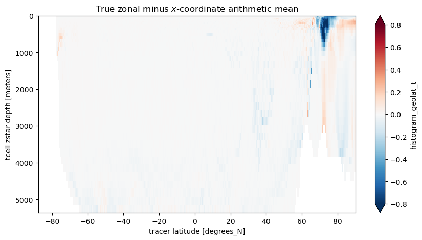
Since we used the same bin edges as the standard yt_ocean coordinate we can take a difference between the arithmetic mean along the model’s x-axis and our mean along grid cells within latitude bands. The main differences are near the North Pole where the grid is furthest for being regular. There are also differences near the Antacrtic Shelf suggesting partial cells also matter.
[13]:
%%timezonal_minus_x_mean=coord_mean.sel(year=2000)-x_arith_mean.sel(year=2000).valuesplt.figure(figsize=(10,5))zonal_minus_x_mean.plot(yincrease=False,vmin=-0.8,vmax=0.8,cmap='RdBu_r',extend='both')plt.title('True zonal minus $x$-coordinate arithmetic mean');
/g/data/xp65/public/apps/med_conda/envs/analysis3-25.09/lib/python3.11/site-packages/distributed/client.py:3363: UserWarning: Sending large graph of size 14.83 MiB.
This may cause some slowdown.
Consider loading the data with Dask directly
 or using futures or delayed objects to embed the data into the graph without repetition.
See also https://docs.dask.org/en/stable/best-practices.html#load-data-with-dask for more information.
  warnings.warn(
/g/data/xp65/public/apps/med_conda/envs/analysis3-25.09/lib/python3.11/site-packages/dask/_task_spec.py:764: RuntimeWarning: invalid value encountered in divide
  return self.func(*new_argspec)
/g/data/xp65/public/apps/med_conda/envs/analysis3-25.09/lib/python3.11/site-packages/dask/_task_spec.py:764: RuntimeWarning: invalid value encountered in divide
  return self.func(*new_argspec)
/g/data/xp65/public/apps/med_conda/envs/analysis3-25.09/lib/python3.11/site-packages/dask/_task_spec.py:764: RuntimeWarning: invalid value encountered in divide
  return self.func(*new_argspec)
/g/data/xp65/public/apps/med_conda/envs/analysis3-25.09/lib/python3.11/site-packages/dask/_task_spec.py:764: RuntimeWarning: invalid value encountered in divide
  return self.func(*new_argspec)
/g/data/xp65/public/apps/med_conda/envs/analysis3-25.09/lib/python3.11/site-packages/dask/_task_spec.py:764: RuntimeWarning: invalid value encountered in divide
  return self.func(*new_argspec)
CPU times: user 6.56 s, sys: 622 ms, total: 7.18 s
Wall time: 7.36 s
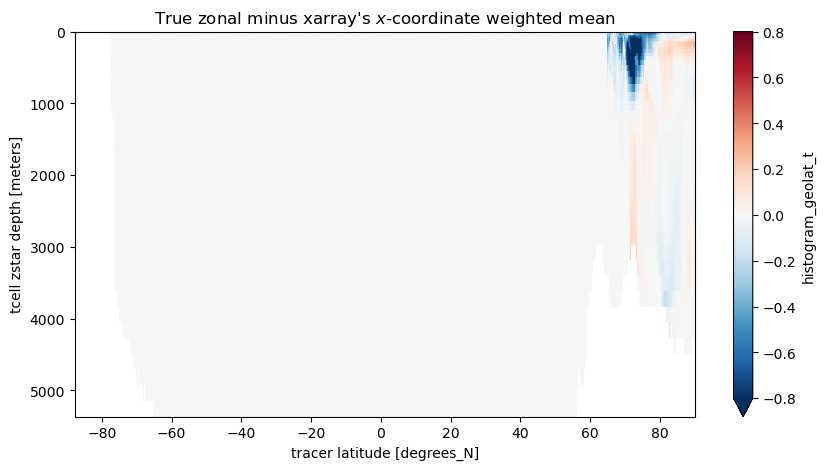
xarray has a new weighted functionality which allows it to do weighted means instead of arithmetic mean.
Let’s see how that works out… We chose dVt as the weights and we only do the comparison for year 2000.
zonal_minus_x_mean=coord_mean.sel(year=2000)-meanweighted_y2000.valuesplt.figure(figsize=(10,5))zonal_minus_x_mean.plot(yincrease=False,vmin=-0.8,vmax=0.8,cmap='RdBu_r')plt.title("True zonal minus xarray's $x$-coordinate weighted mean");
/g/data/xp65/public/apps/med_conda/envs/analysis3-25.09/lib/python3.11/site-packages/distributed/client.py:3363: UserWarning: Sending large graph of size 14.83 MiB.
This may cause some slowdown.
Consider loading the data with Dask directly
 or using futures or delayed objects to embed the data into the graph without repetition.
See also https://docs.dask.org/en/stable/best-practices.html#load-data-with-dask for more information.
  warnings.warn(
/g/data/xp65/public/apps/med_conda/envs/analysis3-25.09/lib/python3.11/site-packages/dask/_task_spec.py:764: RuntimeWarning: invalid value encountered in divide
  return self.func(*new_argspec)
/g/data/xp65/public/apps/med_conda/envs/analysis3-25.09/lib/python3.11/site-packages/dask/_task_spec.py:764: RuntimeWarning: invalid value encountered in divide
  return self.func(*new_argspec)
/g/data/xp65/public/apps/med_conda/envs/analysis3-25.09/lib/python3.11/site-packages/dask/_task_spec.py:764: RuntimeWarning: invalid value encountered in divide
  return self.func(*new_argspec)
/g/data/xp65/public/apps/med_conda/envs/analysis3-25.09/lib/python3.11/site-packages/dask/_task_spec.py:764: RuntimeWarning: invalid value encountered in divide
  return self.func(*new_argspec)
/g/data/xp65/public/apps/med_conda/envs/analysis3-25.09/lib/python3.11/site-packages/dask/_task_spec.py:764: RuntimeWarning: invalid value encountered in divide
  return self.func(*new_argspec)
South of 65N, where complications of the tripolar grid don’t matter, xarray’s weighted mean does the job! But in the region of the tripolar we need to be more careful.