Querying Scalar Quantities and Annually Averaged Timeseries
Models compute globally averaged quantities that are stored in ocean_scalars.nc files. This notebook shows how we do data discovery on scalar quantities and plot them as time series.
Requirements: conda/analysis3-22.10 (or later).
[1]:
%matplotlib inline

import cosima_cookbook as cc
import pandas as pd
import matplotlib.pyplot as plt
from dask.distributed import Client
It’s often a good idea to start a cluster with multiple cores for you to work with.
[2]:
client = Client(n_workers=4)
client
[2]:
Client
Client-a3d7aefe-b3d0-11ed-af57-00000757fe80
| Connection method: Cluster object | Cluster type: distributed.LocalCluster |
| Dashboard: /proxy/8787/status |
Cluster Info
LocalCluster
e4acb176
| Dashboard: /proxy/8787/status | Workers: 4 |
| Total threads: 4 | Total memory: 50.00 GiB |
| Status: running | Using processes: True |
Scheduler Info
Scheduler
Scheduler-c4120003-b70a-4c7c-b31c-d1f44fabd186
| Comm: tcp://127.0.0.1:43271 | Workers: 4 |
| Dashboard: /proxy/8787/status | Total threads: 4 |
| Started: Just now | Total memory: 50.00 GiB |
Workers
Worker: 0
| Comm: tcp://127.0.0.1:44335 | Total threads: 1 |
| Dashboard: /proxy/43529/status | Memory: 12.50 GiB |
| Nanny: tcp://127.0.0.1:39469 | |
| Local directory: /jobfs/73839052.gadi-pbs/dask-worker-space/worker-l0m7278o | |
Worker: 1
| Comm: tcp://127.0.0.1:38733 | Total threads: 1 |
| Dashboard: /proxy/42985/status | Memory: 12.50 GiB |
| Nanny: tcp://127.0.0.1:46127 | |
| Local directory: /jobfs/73839052.gadi-pbs/dask-worker-space/worker-imndlu_t | |
Worker: 2
| Comm: tcp://127.0.0.1:39775 | Total threads: 1 |
| Dashboard: /proxy/44347/status | Memory: 12.50 GiB |
| Nanny: tcp://127.0.0.1:46705 | |
| Local directory: /jobfs/73839052.gadi-pbs/dask-worker-space/worker-b60drufz | |
Worker: 3
| Comm: tcp://127.0.0.1:36281 | Total threads: 1 |
| Dashboard: /proxy/40663/status | Memory: 12.50 GiB |
| Nanny: tcp://127.0.0.1:42701 | |
| Local directory: /jobfs/73839052.gadi-pbs/dask-worker-space/worker-hn00qgol | |
Querying Scalar Quantities
Connect to the default database:
[3]:
session = cc.database.create_session()
An experiment is a particular model run with a given forcing. It is composed of several independent runs of the model.
Here is a list of experiments from the 0.25 degree ACCESS-OM2 physics only global configuration with JRA55-do v1.4 IAF Interannual Forcing, following the OMIP-2 protocol, and with at least 2000 NetCDF files.
[4]:
df = cc.querying.get_experiments(session)
df[df['experiment'].str.contains("025deg_jra55_iaf_omip2_cycle") & (df.ncfiles >1000)]
[4]:
| experiment | ncfiles | |
|---|---|---|
| 41 | 025deg_jra55_iaf_omip2_cycle5 | 2171 |
| 95 | 025deg_jra55_iaf_omip2_cycle1 | 2171 |
| 120 | 025deg_jra55_iaf_omip2_cycle3 | 2210 |
| 121 | 025deg_jra55_iaf_omip2_cycle2 | 2171 |
| 122 | 025deg_jra55_iaf_omip2_cycle6 | 2171 |
| 123 | 025deg_jra55_iaf_omip2_cycle4 | 2171 |
| 167 | 025deg_jra55_iaf_omip2_cycle6_ext | 1570 |
| 168 | 025deg_jra55_iaf_omip2_cycle6_14to17 | 3042 |
| 169 | 025deg_jra55_iaf_omip2_cycle6_78to08 | 5860 |
An experiment is composed of many different variables which are stored at different frequencies.
The function cc.querying.get_frequencies gives a list of the frequencies are available for a particular experiment.
[5]:
cc.querying.get_frequencies(session, "025deg_jra55_iaf_omip2_cycle5")
[5]:
| frequency | |
|---|---|
| 0 | None |
| 1 | 1 daily |
| 2 | 1 monthly |
| 3 | 1 yearly |
| 4 | static |
Here are all of the variables that are stored at the frequency of 1 monthly and also are files of the form ocean/ocean_scalar.nc.
[6]:
pd.set_option("display.max_rows", 200) # to ensure all rows of the pandas DataFrame are displayed
df = cc.querying.get_variables(session, "025deg_jra55_iaf_omip2_cycle5",
                               frequency = "1 monthly")
df[df.ncfile.str.contains("ocean_scalar.nc")]
[6]:
| name | long_name | units | frequency | ncfile | cell_methods | # ncfiles | time_start | time_end | |
|---|---|---|---|---|---|---|---|---|---|
| 20 | average_DT | Length of average period | days | 1 monthly | output153/ocean/ocean_scalar.nc | None | 308 | 1957-12-30 00:00:00 | 2257-12-30 00:00:00 |
| 21 | average_T1 | Start time for average period | days since 0001-01-01 00:00:00 | 1 monthly | output153/ocean/ocean_scalar.nc | None | 308 | 1957-12-30 00:00:00 | 2257-12-30 00:00:00 |
| 22 | average_T2 | End time for average period | days since 0001-01-01 00:00:00 | 1 monthly | output153/ocean/ocean_scalar.nc | None | 308 | 1957-12-30 00:00:00 | 2257-12-30 00:00:00 |
| 36 | eta_global | global ave eta_t plus patm_t/(g*rho0) | meter | 1 monthly | output153/ocean/ocean_scalar.nc | time: mean | 154 | 1957-12-30 00:00:00 | 2257-12-30 00:00:00 |
| 64 | ke_tot | Globally integrated ocean kinetic energy | 10^15 Joules | 1 monthly | output153/ocean/ocean_scalar.nc | time: mean | 154 | 1957-12-30 00:00:00 | 2257-12-30 00:00:00 |
| 75 | nv | vertex number | none | 1 monthly | output153/ocean/ocean_scalar.nc | None | 308 | 1957-12-30 00:00:00 | 2257-12-30 00:00:00 |
| 77 | pe_tot | Globally integrated ocean potential energy | 10^15 Joules | 1 monthly | output153/ocean/ocean_scalar.nc | time: mean | 154 | 1957-12-30 00:00:00 | 2257-12-30 00:00:00 |
| 81 | rhoave | global mean ocean in-situ density from ocean_d... | kg/m^3 | 1 monthly | output153/ocean/ocean_scalar.nc | time: mean | 154 | 1957-12-30 00:00:00 | 2257-12-30 00:00:00 |
| 85 | salt_global_ave | Global mean salt in liquid seawater | psu | 1 monthly | output153/ocean/ocean_scalar.nc | time: mean | 154 | 1957-12-30 00:00:00 | 2257-12-30 00:00:00 |
| 86 | salt_surface_ave | Global mass weighted mean surface salt in liqu... | psu | 1 monthly | output153/ocean/ocean_scalar.nc | time: mean | 154 | 1957-12-30 00:00:00 | 2257-12-30 00:00:00 |
| 87 | scalar_axis | none | none | 1 monthly | output153/ocean/ocean_scalar.nc | None | 154 | 1957-12-30 00:00:00 | 2257-12-30 00:00:00 |
| 125 | temp_global_ave | Global mean temp in liquid seawater | deg_C | 1 monthly | output153/ocean/ocean_scalar.nc | time: mean | 154 | 1957-12-30 00:00:00 | 2257-12-30 00:00:00 |
| 129 | temp_surface_ave | Global mass weighted mean surface temp in liqu... | deg_C | 1 monthly | output153/ocean/ocean_scalar.nc | time: mean | 154 | 1957-12-30 00:00:00 | 2257-12-30 00:00:00 |
| 145 | time | time | days since 0001-01-01 00:00:00 | 1 monthly | output153/ocean/ocean_scalar.nc | None | 462 | 1957-12-30 00:00:00 | 2257-12-30 00:00:00 |
| 147 | time_bounds | time axis boundaries | days | 1 monthly | output153/ocean/ocean_scalar.nc | None | 308 | 1957-12-30 00:00:00 | 2257-12-30 00:00:00 |
| 150 | total_net_sfc_heating | total ocean surface flux from coupler and mass... | Watts/1e15 | 1 monthly | output153/ocean/ocean_scalar.nc | time: mean | 154 | 1957-12-30 00:00:00 | 2257-12-30 00:00:00 |
| 151 | total_ocean_calving | total water entering ocean from calving land ice | (kg/sec)/1e15 | 1 monthly | output153/ocean/ocean_scalar.nc | time: mean | 154 | 1957-12-30 00:00:00 | 2257-12-30 00:00:00 |
| 152 | total_ocean_calving_heat | total ocean heat flux from calving land ice | Watts/1e15 | 1 monthly | output153/ocean/ocean_scalar.nc | time: mean | 154 | 1957-12-30 00:00:00 | 2257-12-30 00:00:00 |
| 153 | total_ocean_calving_melt_heat | total heat flux to melt frozen land ice (<0 co... | Watts/1e15 | 1 monthly | output153/ocean/ocean_scalar.nc | time: mean | 154 | 1957-12-30 00:00:00 | 2257-12-30 00:00:00 |
| 154 | total_ocean_evap | total evaporative ocean mass flux (>0 enters o... | (kg/sec)/1e15 | 1 monthly | output153/ocean/ocean_scalar.nc | time: mean | 154 | 1957-12-30 00:00:00 | 2257-12-30 00:00:00 |
| 155 | total_ocean_evap_heat | total latent heat flux into ocean (<0 cools oc... | Watts/1e15 | 1 monthly | output153/ocean/ocean_scalar.nc | time: mean | 154 | 1957-12-30 00:00:00 | 2257-12-30 00:00:00 |
| 156 | total_ocean_fprec | total snow falling onto ocean (>0 enters ocean) | (kg/sec)/1e15 | 1 monthly | output153/ocean/ocean_scalar.nc | time: mean | 154 | 1957-12-30 00:00:00 | 2257-12-30 00:00:00 |
| 157 | total_ocean_fprec_melt_heat | total heat flux to melt frozen precip (<0 cool... | Watts/1e15 | 1 monthly | output153/ocean/ocean_scalar.nc | time: mean | 154 | 1957-12-30 00:00:00 | 2257-12-30 00:00:00 |
| 158 | total_ocean_heat | Total heat in the liquid ocean referenced to 0... | Joule/1e25 | 1 monthly | output153/ocean/ocean_scalar.nc | time: mean | 154 | 1957-12-30 00:00:00 | 2257-12-30 00:00:00 |
| 159 | total_ocean_hflux_coupler | total surface heat flux passed through coupler | Watts/1e15 | 1 monthly | output153/ocean/ocean_scalar.nc | time: mean | 154 | 1957-12-30 00:00:00 | 2257-12-30 00:00:00 |
| 160 | total_ocean_hflux_evap | total ocean heat flux from evap transferring w... | Watts/1e15 | 1 monthly | output153/ocean/ocean_scalar.nc | time: mean | 154 | 1957-12-30 00:00:00 | 2257-12-30 00:00:00 |
| 161 | total_ocean_hflux_prec | total ocean heat flux from precip transferring... | Watts/1e15 | 1 monthly | output153/ocean/ocean_scalar.nc | time: mean | 154 | 1957-12-30 00:00:00 | 2257-12-30 00:00:00 |
| 162 | total_ocean_lprec | total liquid precip into ocean (>0 enters ocean) | (kg/sec)/1e15 | 1 monthly | output153/ocean/ocean_scalar.nc | time: mean | 154 | 1957-12-30 00:00:00 | 2257-12-30 00:00:00 |
| 163 | total_ocean_lw_heat | total longwave flux into ocean (<0 cools ocean) | Watts/1e15 | 1 monthly | output153/ocean/ocean_scalar.nc | time: mean | 154 | 1957-12-30 00:00:00 | 2257-12-30 00:00:00 |
| 164 | total_ocean_melt | total liquid water melted from sea ice (>0 ent... | (kg/sec)/1e15 | 1 monthly | output153/ocean/ocean_scalar.nc | time: mean | 154 | 1957-12-30 00:00:00 | 2257-12-30 00:00:00 |
| 165 | total_ocean_pme_river | total ocean precip-evap+river via sbc (liquid,... | (kg/sec)/1e15 | 1 monthly | output153/ocean/ocean_scalar.nc | time: mean | 154 | 1957-12-30 00:00:00 | 2257-12-30 00:00:00 |
| 166 | total_ocean_river | total liquid river water and calving ice enter... | kg/sec/1e15 | 1 monthly | output153/ocean/ocean_scalar.nc | time: mean | 154 | 1957-12-30 00:00:00 | 2257-12-30 00:00:00 |
| 167 | total_ocean_river_heat | total heat flux into ocean from liquid+solid r... | Watts/1e15 | 1 monthly | output153/ocean/ocean_scalar.nc | time: mean | 154 | 1957-12-30 00:00:00 | 2257-12-30 00:00:00 |
| 168 | total_ocean_runoff | total liquid river runoff (>0 water enters ocean) | (kg/sec)/1e15 | 1 monthly | output153/ocean/ocean_scalar.nc | time: mean | 154 | 1957-12-30 00:00:00 | 2257-12-30 00:00:00 |
| 169 | total_ocean_runoff_heat | total ocean heat flux from liquid river runoff | Watts/1e15 | 1 monthly | output153/ocean/ocean_scalar.nc | time: mean | 154 | 1957-12-30 00:00:00 | 2257-12-30 00:00:00 |
| 170 | total_ocean_salt | total mass of salt in liquid seawater | kg/1e18 | 1 monthly | output153/ocean/ocean_scalar.nc | time: mean | 154 | 1957-12-30 00:00:00 | 2257-12-30 00:00:00 |
| 171 | total_ocean_sens_heat | total sensible heat into ocean (<0 cools ocean) | Watts/1e15 | 1 monthly | output153/ocean/ocean_scalar.nc | time: mean | 154 | 1957-12-30 00:00:00 | 2257-12-30 00:00:00 |
| 172 | total_ocean_sfc_salt_flux_coupler | total_ocean_sfc_salt_flux_coupler | kg/sec (*1e-15) | 1 monthly | output153/ocean/ocean_scalar.nc | time: mean | 154 | 1957-12-30 00:00:00 | 2257-12-30 00:00:00 |
| 173 | total_ocean_swflx | total shortwave flux into ocean (>0 heats ocean) | Watts/1e15 | 1 monthly | output153/ocean/ocean_scalar.nc | time: mean | 154 | 1957-12-30 00:00:00 | 2257-12-30 00:00:00 |
| 174 | total_ocean_swflx_vis | total visible shortwave into ocean (>0 heats o... | Watts/1e15 | 1 monthly | output153/ocean/ocean_scalar.nc | time: mean | 154 | 1957-12-30 00:00:00 | 2257-12-30 00:00:00 |
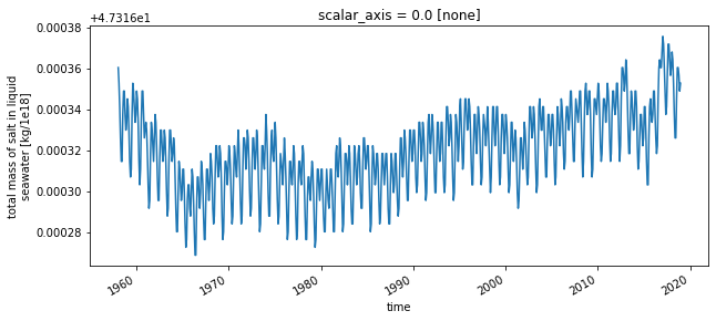
Say, we want to look at one of these variables such as “total_ocean_salt”. We use cc.querying.getvar() for this.
[7]:
experiment = "025deg_jra55_iaf_omip2_cycle5"
variable = "total_ocean_salt"
da = cc.querying.getvar(experiment, variable, session,ncfile='ocean_scalar.nc')
da
[7]:
<xarray.DataArray 'total_ocean_salt' (time: 732, scalar_axis: 1)>
dask.array<concatenate, shape=(732, 1), dtype=float32, chunksize=(1, 1), chunktype=numpy.ndarray>
Coordinates:
  * scalar_axis  (scalar_axis) float64 0.0
  * time         (time) datetime64[ns] 1958-01-14T12:00:00 ... 2018-12-14T12:...
Attributes:
    long_name:      total mass of salt in liquid seawater
    units:          kg/1e18
    valid_range:    [-1.e+02  1.e+10]
    cell_methods:   time: mean
    time_avg_info:  average_T1,average_T2,average_DT
    ncfiles:        ['/g/data/ik11/outputs/access-om2-025/025deg_jra55_iaf_om...
    contact:        Ryan Holmes
    email:          ryan.holmes@unsw.edu.au
    created:        2020-11-03
description: 0.25 degree ACCESS-OM2 global model configuration under i...[8]:
da.plot(figsize=(10,4))
[8]:
[<matplotlib.lines.Line2D at 0x15467df5a9d0>]
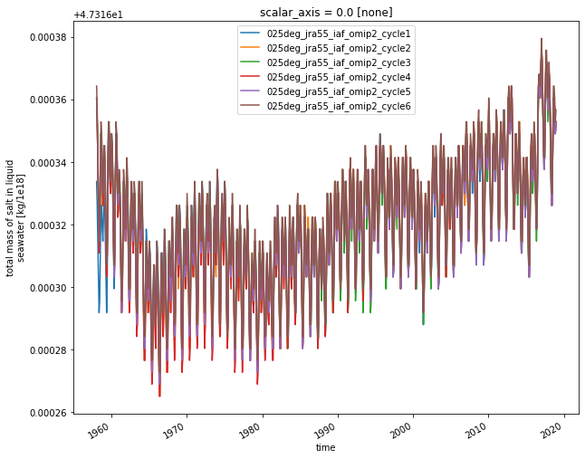
Suppose we want to compare this variable across several different experiments. Using our list of experiments from above, we call put that into a Python list.
Here we select the six 61-year cycles of 1 Jan 1958 to 1 Jan 2019 from the list of experiments above. These cycles are sequential, with each cycle starting where the previous one ended, with the initialization date reset to 1959. Here we show how to plot some quantities to compare those cycles.
[9]:
df = cc.querying.get_experiments(session)
experiments = list(df[df['experiment'].str.contains("025deg_jra55_iaf_omip2_cycle") &
   (df.ncfiles > 1000)].experiment)
experiments = sorted(experiments[:6])
experiments
[9]:
['025deg_jra55_iaf_omip2_cycle1',
 '025deg_jra55_iaf_omip2_cycle2',
 '025deg_jra55_iaf_omip2_cycle3',
 '025deg_jra55_iaf_omip2_cycle4',
 '025deg_jra55_iaf_omip2_cycle5',
 '025deg_jra55_iaf_omip2_cycle6']
And for each experiment, extract out the variable of interest and store the result in a dictionary using the experiment as the key. Notice we are computing the variables and storing the results for later visualization.
Here we add an exception for experiments that do not have total_ocean_salt as an output
[10]:
results = {}
variable = "total_ocean_salt"
for experiment in experiments:
  try:
    results[experiment] = cc.querying.getvar(experiment, variable, session, ncfile="ocean_scalar.nc")
  except cc.querying.VariableNotFoundError:
    print(f"No {variable} in {experiment}")
Now, plot the results
[11]:
fig, ax = plt.subplots(1, 1, figsize=(10, 8))
for experiment, result in results.items():
    result.plot(label=experiment, ax=ax)
ax.legend()
[11]:
<matplotlib.legend.Legend at 0x154674eccbe0>
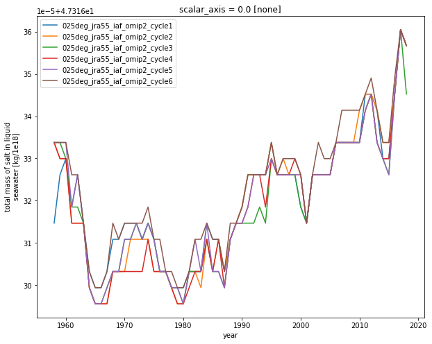
Annually Averaged Scalar Timeseries
This section presents how the data are resampled onto annual averages.
Note that the previous timeseries are monthly so we need to use groupby and a time mean to resample the data onto annual frequency.
[12]:
results_annual_average = dict()
for experiment, result in results.items():
    results_annual_average[experiment] = results[experiment].groupby('time.year').mean(dim='time')
Then, the data can be plotted as you see fit:
[13]:
fig, ax = plt.subplots(1, 1, figsize=(10, 8))
for experiment, result_annual_average in results_annual_average.items():
    result_annual_average.plot(label = experiment)
ax.legend()
[13]:
<matplotlib.legend.Legend at 0x15466fea6eb0>