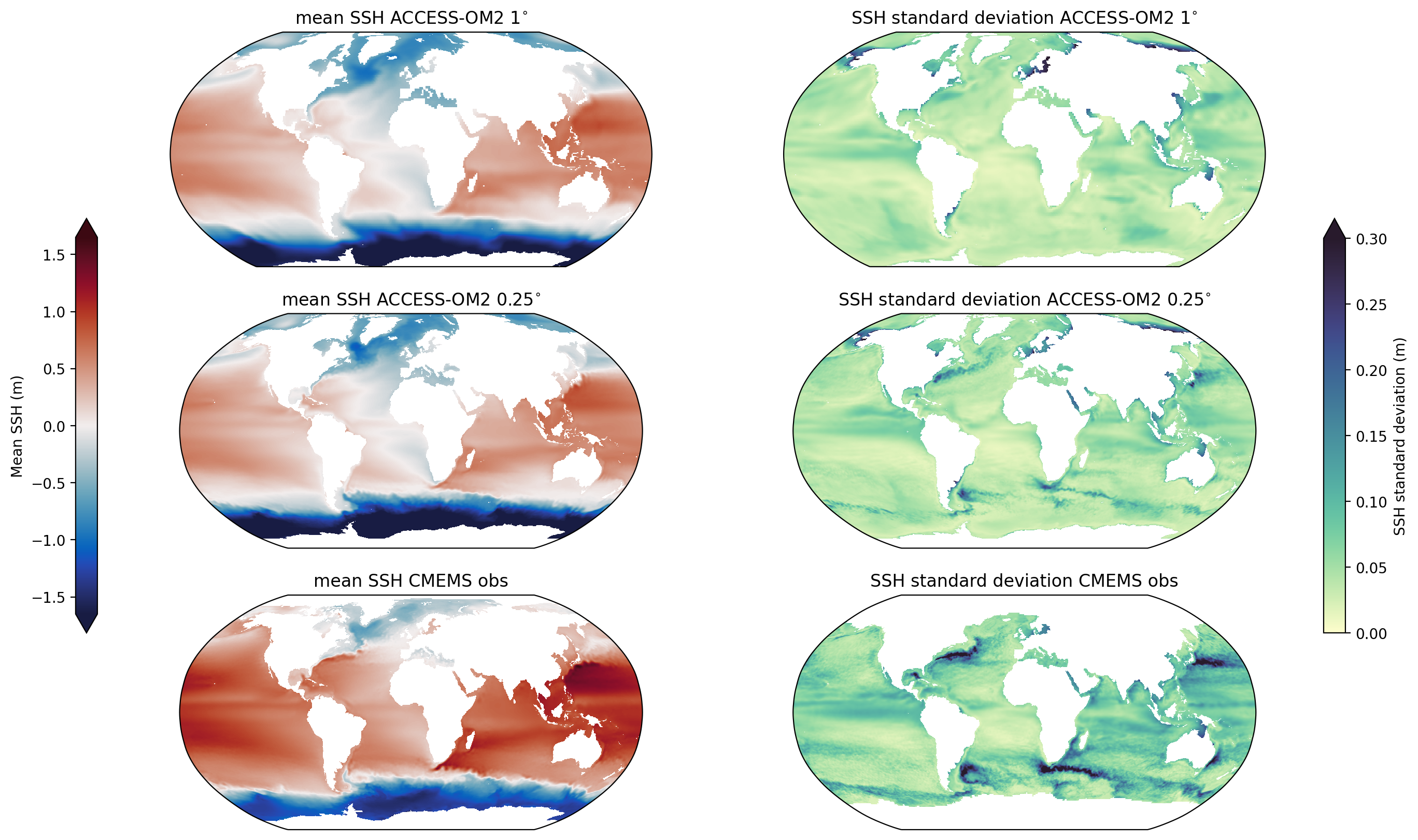
Compare sea surface height model output and observations
Comparing the sea-surface height (ssh) from two different resolution runs. Specifically, we plot the time-mean and standard deviation of ssh and compare it to those obtained from observations from the CMEMS satellite altimetry dataset (former AVISO+ dataset).
[1]:
%matplotlib inline
%config InlineBackend.figure_format='retina'

import matplotlib.pyplot as plt
import cosima_cookbook as cc
import numpy as np
import glob

import xarray as xr
import cartopy.crs as ccrs
import cmocean as cm

from dask.distributed import Client
[2]:
client = Client()
client
[2]:
Client
Client-791aa755-a349-11ed-97a5-00000777fe80
| Connection method: Cluster object | Cluster type: distributed.LocalCluster |
| Dashboard: /proxy/8787/status |
Cluster Info
LocalCluster
bb7ca7cb
| Dashboard: /proxy/8787/status | Workers: 7 |
| Total threads: 28 | Total memory: 112.00 GiB |
| Status: running | Using processes: True |
Scheduler Info
Scheduler
Scheduler-e0f69a79-68bb-46c5-99ba-9058c27e46ce
| Comm: tcp://127.0.0.1:43535 | Workers: 7 |
| Dashboard: /proxy/8787/status | Total threads: 28 |
| Started: Just now | Total memory: 112.00 GiB |
Workers
Worker: 0
| Comm: tcp://127.0.0.1:39535 | Total threads: 4 |
| Dashboard: /proxy/42459/status | Memory: 16.00 GiB |
| Nanny: tcp://127.0.0.1:36119 | |
| Local directory: /jobfs/71378961.gadi-pbs/dask-worker-space/worker-by7qqmth | |
Worker: 1
| Comm: tcp://127.0.0.1:34005 | Total threads: 4 |
| Dashboard: /proxy/37755/status | Memory: 16.00 GiB |
| Nanny: tcp://127.0.0.1:41341 | |
| Local directory: /jobfs/71378961.gadi-pbs/dask-worker-space/worker-y29a1vwg | |
Worker: 2
| Comm: tcp://127.0.0.1:37607 | Total threads: 4 |
| Dashboard: /proxy/45849/status | Memory: 16.00 GiB |
| Nanny: tcp://127.0.0.1:39259 | |
| Local directory: /jobfs/71378961.gadi-pbs/dask-worker-space/worker-ws8ze_2z | |
Worker: 3
| Comm: tcp://127.0.0.1:38735 | Total threads: 4 |
| Dashboard: /proxy/38235/status | Memory: 16.00 GiB |
| Nanny: tcp://127.0.0.1:42225 | |
| Local directory: /jobfs/71378961.gadi-pbs/dask-worker-space/worker-ryhvrakh | |
Worker: 4
| Comm: tcp://127.0.0.1:36141 | Total threads: 4 |
| Dashboard: /proxy/46077/status | Memory: 16.00 GiB |
| Nanny: tcp://127.0.0.1:34177 | |
| Local directory: /jobfs/71378961.gadi-pbs/dask-worker-space/worker-ava4xcpr | |
Worker: 5
| Comm: tcp://127.0.0.1:36587 | Total threads: 4 |
| Dashboard: /proxy/45669/status | Memory: 16.00 GiB |
| Nanny: tcp://127.0.0.1:34409 | |
| Local directory: /jobfs/71378961.gadi-pbs/dask-worker-space/worker-em80j705 | |
Worker: 6
| Comm: tcp://127.0.0.1:35037 | Total threads: 4 |
| Dashboard: /proxy/35677/status | Memory: 16.00 GiB |
| Nanny: tcp://127.0.0.1:33101 | |
| Local directory: /jobfs/71378961.gadi-pbs/dask-worker-space/worker-zl7uf2ke | |
Start a cookbook database session
[3]:
session = cc.database.create_session()
Here we pick a start_time and end_time. We select only 5 years of daily data for simplicity in this example. But you can probably extend the end_time until the end of 2018 (for model outputs) and up to middle of 2020 for observations!
[4]:
#SSH variable in ACCESS-OM2 models
variable = 'sea_level'

start_time = '1993-01-01'
end_time = '1997-12-31'
SSH from 1\(^{\circ}\) model output
Here we can specify the rough start and end times using the start_time and end_time arguments. After we load them, we slice the data in time to ensure we have the same time range in all datasets we plan to compare.
[5]:
experiment = '1deg_jra55_iaf_omip2_cycle6'  # 1-deg experiment
ssh1 = cc.querying.getvar(experiment, variable, session, frequency='1 daily',
                          start_time=start_time, end_time=end_time)
ssh1 = ssh1.sel(time=slice(start_time, end_time))
ssh1
[5]:
<xarray.DataArray 'sea_level' (time: 1826, yt_ocean: 300, xt_ocean: 360)>
dask.array<getitem, shape=(1826, 300, 360), dtype=float32, chunksize=(1, 300, 360), chunktype=numpy.ndarray>
Coordinates:
  * xt_ocean  (xt_ocean) float64 -279.5 -278.5 -277.5 -276.5 ... 77.5 78.5 79.5
  * yt_ocean  (yt_ocean) float64 -77.88 -77.63 -77.38 ... 88.87 89.32 89.77
  * time      (time) datetime64[ns] 1993-01-01T12:00:00 ... 1997-12-31T12:00:00
Attributes:
    long_name:      effective sea level (eta_t + patm/(rho0*g)) on T cells
    units:          meter
    valid_range:    [-1000.  1000.]
    cell_methods:   time: mean
    time_avg_info:  average_T1,average_T2,average_DT
    coordinates:    geolon_t geolat_t
    standard_name:  sea_surface_height_above_geoid
    ncfiles:        ['/g/data/ik11/outputs/access-om2/1deg_jra55_iaf_omip2_cy...
    contact:        Hakase Hayashida
    email:          hakase.hayashida@utas.edu.au
    created:        2021-03-03
description: 1 degree ACCESS-OM2 global model configuration under inte...SSH from 0.25\(^{\circ}\) model output
[6]:
experiment = '025deg_jra55_iaf_omip2_cycle6'  # 0.25-deg experiment
ssh025 = cc.querying.getvar(experiment, variable, session, frequency='1 daily',
                            start_time=start_time, end_time=end_time)
ssh025 = ssh025.sel(time=slice(start_time, end_time))
ssh025
[6]:
<xarray.DataArray 'sea_level' (time: 1826, yt_ocean: 1080, xt_ocean: 1440)>
dask.array<getitem, shape=(1826, 1080, 1440), dtype=float32, chunksize=(1, 216, 240), chunktype=numpy.ndarray>
Coordinates:
  * xt_ocean  (xt_ocean) float64 -279.9 -279.6 -279.4 ... 79.38 79.62 79.88
  * yt_ocean  (yt_ocean) float64 -81.08 -80.97 -80.87 ... 89.74 89.84 89.95
  * time      (time) datetime64[ns] 1993-01-01T12:00:00 ... 1997-12-31T12:00:00
Attributes:
    long_name:      effective sea level (eta_t + patm/(rho0*g)) on T cells
    units:          meter
    valid_range:    [-1000.  1000.]
    cell_methods:   time: mean
    time_avg_info:  average_T1,average_T2,average_DT
    coordinates:    geolon_t geolat_t
    standard_name:  sea_surface_height_above_geoid
    ncfiles:        ['/g/data/ik11/outputs/access-om2-025/025deg_jra55_iaf_om...
    contact:        Ryan Holmes
    email:          ryan.holmes@unsw.edu.au
    created:        2020-11-03
description: 0.25 degree ACCESS-OM2 global model configuration under i...CMEMS satellite observational data (former AVISO+ dataset)
Load the CMEMS dataset and select adt the sea surface height variable name.
Note: You need to join project ua8 on NCI to access the CMEMS data!
[7]:
filenames = glob.glob("/g/data/ua8/CMEMS_SeaLevel/timeseries/*.nc")
cmems = xr.open_mfdataset(filenames, parallel=True)

obs_ssh = cmems.adt
obs_ssh = obs_ssh.sel(time=slice(start_time, end_time))
obs_ssh = obs_ssh.rename('adt_cmems')
obs_ssh
[7]:
<xarray.DataArray 'adt_cmems' (time: 1826, latitude: 720, longitude: 1440)>
dask.array<getitem, shape=(1826, 720, 1440), dtype=float64, chunksize=(366, 720, 1440), chunktype=numpy.ndarray>
Coordinates:
  * time       (time) datetime64[ns] 1993-01-01 1993-01-02 ... 1997-12-31
  * longitude  (longitude) float32 0.125 0.375 0.625 0.875 ... 359.4 359.6 359.9
  * latitude   (latitude) float32 -89.88 -89.62 -89.38 ... 89.38 89.62 89.88
Attributes:
    standard_name:  sea_surface_height_above_geoid
    long_name:      Absolute dynamic topography
    units:          m
    grid_mapping:   crs
comment: The absolute dynamic topography is the sea surface height...Compute the mean and standard deviations to plot. We add .load() so to enforce computations. For the std calculations we provide skipna=False option to tell xarray to ignore the points on land that have NaN values. This way it doesn’t try to divide by a zero-length series while computing the standard deviation. (If we didn’t provideskipna=False we’d get the same answer but with a bunch of RuntimeWarnings.)
Note: The following cells might take a while, depending how much data you loaded. (for 5 years of daily data ~7min for 0.25 model output using 28 cpus).
[8]:
%%time
ssh1_mean = ssh1.mean(dim='time').load()
ssh1_std  = ssh1.std(dim='time', skipna=False).load()
CPU times: user 7.04 s, sys: 358 ms, total: 7.4 s
Wall time: 8.44 s
[9]:
%%time
ssh025_mean = ssh025.mean(dim='time').load()
ssh025_std  = ssh025.std(dim='time', skipna=False).load()
CPU times: user 5min 17s, sys: 9.09 s, total: 5min 26s
Wall time: 5min 28s
[10]:
%%time
obs_ssh_mean = obs_ssh.mean(dim='time').load()
obs_ssh_std  = obs_ssh.std(dim='time', skipna=False).load()
CPU times: user 8.01 s, sys: 938 ms, total: 8.95 s
Wall time: 53 s
Plot and compare
Plot the time-mean and standard deviation of both of the model outputs and the CMEMS observational dataset (former AVISO+).
[11]:
projection = ccrs.Robinson(central_longitude=-100)

fig, axes = plt.subplots(nrows = 3, ncols = 2, figsize = (14, 10),
                         subplot_kw={'projection': ccrs.Robinson()})

max_std = 0.3
max_mean = 1.65

# mean SSH plots
ax = axes[0, 0]
p1 = ssh1_mean.plot(ax=ax, transform=ccrs.PlateCarree(),
                    cmap=cm.cm.balance, vmin=-max_mean, vmax=max_mean, add_colorbar=False)
ax.set_title('mean SSH ACCESS-OM2 1$^{\circ}$')

ax = axes[1, 0]
p1 = ssh025_mean.plot(ax=ax, transform=ccrs.PlateCarree(),
                      cmap=cm.cm.balance, vmin=-max_mean, vmax=max_mean, add_colorbar=False)
ax.set_title('mean SSH ACCESS-OM2 0.25$^{\circ}$')

ax = axes[2, 0]
p1 = obs_ssh_mean.plot(ax=ax, transform=ccrs.PlateCarree(),
                       cmap=cm.cm.balance, vmin=-max_mean, vmax=max_mean, add_colorbar=False)
ax.set_title('mean SSH CMEMS obs')

# std SSH plots
ax = axes[0, 1]
p2 = ssh1_std.plot(ax=ax, transform=ccrs.PlateCarree(),
                   cmap=cm.cm.deep, vmin=0, vmax=max_std, add_colorbar=False)
ax.set_title('SSH standard deviation ACCESS-OM2 1$^{\circ}$')

ax = axes[1, 1]
p2 = ssh025_std.plot(ax=ax, transform=ccrs.PlateCarree(),
                     cmap=cm.cm.deep, vmin=0, vmax=max_std, add_colorbar=False)
ax.set_title('SSH standard deviation ACCESS-OM2 0.25$^{\circ}$')

ax = axes[2, 1]
p2 = obs_ssh_std.plot(ax=ax, transform=ccrs.PlateCarree(),
                      cmap=cm.cm.deep, vmin=0, vmax=max_std, add_colorbar=False)
ax.set_title('SSH standard deviation CMEMS obs')

# Colorbars
ax_cb1 = plt.axes([0.07, 0.3, 0.015, 0.4])
cb = plt.colorbar(p1, cax=ax_cb1, extend='both', label='Mean SSH (m)')
ax_cb1.yaxis.set_ticks_position('left')
ax_cb1.yaxis.set_label_position('left')

ax_cb2 = plt.axes([0.93, 0.3, 0.015, 0.4])
cb = plt.colorbar(p2, cax=ax_cb2, extend='max', label='SSH standard deviation (m)');