Bathymetry
A simple example to show how to plot the model bathymetry for ACCESS-OM2 configurations.
[1]:
%matplotlib inline

import cosima_cookbook as cc
import matplotlib.pyplot as plt
import numpy as np
import xarray as xr
import cmocean as cm
import cartopy.crs as ccrs
from dask.distributed import Client
Start dask cluster:
[2]:
client = Client()
client
[2]:
Client
Client-6863479d-9c5c-11ed-bafc-00000754fe80
| Connection method: Cluster object | Cluster type: distributed.LocalCluster |
| Dashboard: /proxy/42821/status |
Cluster Info
LocalCluster
6768223a
| Dashboard: /proxy/42821/status | Workers: 4 |
| Total threads: 12 | Total memory: 48.00 GiB |
| Status: running | Using processes: True |
Scheduler Info
Scheduler
Scheduler-83518999-9057-444a-9b63-4c61d9766e86
| Comm: tcp://127.0.0.1:38797 | Workers: 4 |
| Dashboard: /proxy/42821/status | Total threads: 12 |
| Started: Just now | Total memory: 48.00 GiB |
Workers
Worker: 0
| Comm: tcp://127.0.0.1:34519 | Total threads: 3 |
| Dashboard: /proxy/36589/status | Memory: 12.00 GiB |
| Nanny: tcp://127.0.0.1:35633 | |
| Local directory: /jobfs/70823302.gadi-pbs/dask-worker-space/worker-4aofncu5 | |
Worker: 1
| Comm: tcp://127.0.0.1:43783 | Total threads: 3 |
| Dashboard: /proxy/34177/status | Memory: 12.00 GiB |
| Nanny: tcp://127.0.0.1:38899 | |
| Local directory: /jobfs/70823302.gadi-pbs/dask-worker-space/worker-8_5_bjrn | |
Worker: 2
| Comm: tcp://127.0.0.1:36409 | Total threads: 3 |
| Dashboard: /proxy/42803/status | Memory: 12.00 GiB |
| Nanny: tcp://127.0.0.1:33391 | |
| Local directory: /jobfs/70823302.gadi-pbs/dask-worker-space/worker-kmomrt3u | |
Worker: 3
| Comm: tcp://127.0.0.1:36293 | Total threads: 3 |
| Dashboard: /proxy/45561/status | Memory: 12.00 GiB |
| Nanny: tcp://127.0.0.1:46761 | |
| Local directory: /jobfs/70823302.gadi-pbs/dask-worker-space/worker-61y3unt4 | |
Connect to the default COSIMA database:
[3]:
session = cc.database.create_session()
First load the bathymetry for your experiment. ‘ht’ is on the t grid. If you want bathymetry on the u grid, use ‘hu’ instead.
[4]:
experiment = '01deg_jra55v140_iaf_cycle3' # or, e.g., '1deg_jra55_iaf_omip2_cycle6' or '025deg_jra55_iaf_omip2_cycle6'

bathymetry = cc.querying.getvar(experiment, 'ht', session, n=1)
Load latitude / longitude data for plotting. We can’t just load geolon_t and geolat_t from this experiment, because those variables have land masks which don’t work with plotting. Make sure the grid file here matches the resolution of the experiment you are looking at. i.e. Use ocean_grid_10.nc if your experiment is 1° or ocean_grid_025.nc for 0.25°.
[5]:
grid = xr.open_dataset('/g/data/ik11/grids/ocean_grid_01.nc')
geolon_t = grid.geolon_t
geolat_t = grid.geolat_t
Create a land mask for plotting, set land cells to 1 and rest to NaN. This is preferred over cartopy.feature, because the land that cartopy.feature provides differs from the model’s land mask.
[6]:
land = xr.where(np.isnan(bathymetry.rename('land')), 1, np.nan)
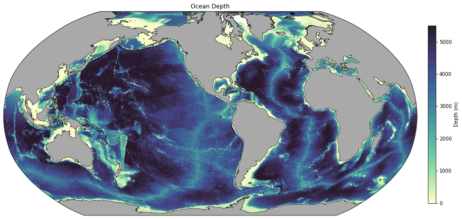
And now plot!
[7]:
fig = plt.figure(figsize=(15, 10))
ax = plt.axes(projection=ccrs.Robinson(central_longitude=-100))

# Add model land mask
land.plot.contourf(ax=ax, colors='darkgrey', zorder=2, transform=ccrs.PlateCarree(), add_colorbar=False)
# Add model coastline
land.fillna(0).plot.contour(ax=ax, colors='k', levels=[0, 1], transform=ccrs.PlateCarree(), add_colorbar=False, linewidths=0.5)

p1 = ax.pcolormesh(geolon_t, geolat_t, bathymetry, transform=ccrs.PlateCarree(), cmap=cm.cm.deep, vmin=0, vmax=5500)
plt.title('Ocean Depth')

ax_cb = plt.axes([0.92, 0.25, 0.015, 0.5])
cb = plt.colorbar(p1, cax=ax_cb, orientation='vertical')
cb.ax.set_ylabel('Depth (m)');
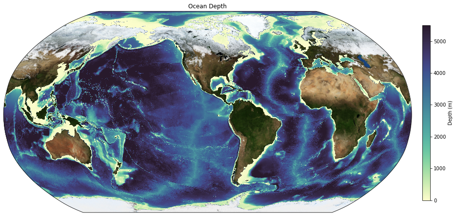
Now let’s add pretty land (NASA Blue Marble):
[8]:
map_path = '/g/data/ik11/grids/BlueMarble.tiff'
blue_marble = plt.imread(map_path)
blue_marble_extent = (-180, 180, -90, 90)
[9]:
fig = plt.figure(figsize=(15, 10))
ax = plt.axes(projection=ccrs.Robinson(central_longitude=-100))

p1 = ax.pcolormesh(geolon_t, geolat_t, bathymetry, transform=ccrs.PlateCarree(), cmap=cm.cm.deep, vmin=0, vmax=5500)
plt.title('Ocean Depth')

# Add pretty land:
ax.imshow(blue_marble, extent=blue_marble_extent, transform=ccrs.PlateCarree(), origin='upper')

# Colorbar:
ax_cb = plt.axes([0.92, 0.25, 0.015, 0.5])
cb = plt.colorbar(p1, cax=ax_cb, orientation='vertical')
cb.ax.set_ylabel('Depth (m)');