Coordinate transformation from z levels to density levels¶

Rebinning `ty_trans` to `ty_trans_rho` density levels¶

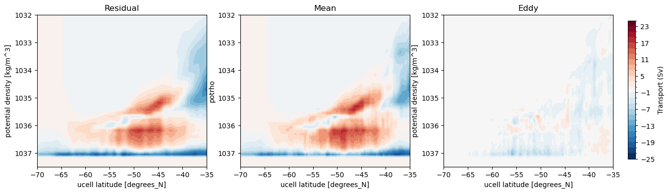
This transformation is commonly used for the purpose of decomposing the residual meridional overturning streamfunction into mean and eddy components. The mean is taken to be the time-mean Eulerian transport (time-mean in z coordinates), whilst the residual transport is the time-mean in density coordinates (density surface move in time). The eddy transport is the difference between the residual overturning streamfunction, and the Eulerian transport transformed from depth to density coordinates via the time-mean density.

Binning is the discrete version of this transformation from depth to density coordinates. We define target density bins, and for each bin we add the quantity to be binned from all cells with a density that satisfies that bin. In its simplest form, binning is creating a histogram.

We use three different binning methods:

xhistogram, which performs binning in exactly the way MOM5 does and is thus most appropriate for calculating eddy quantities (define edge of bins)
xgcm conservative binning (define edge of bins, but vertically interpolates so looks smoother than xhistogram)
Using density coordinate binning method of Lee et al. (2007) (define isopycnals to bin onto i.e. centre)

Compute times were calculated using the XXLarge (28 cpus, 128 Gb mem) Jupyter Lab on NCI’s ARE, using conda environment analysis3-25.05.

This notebook performs direct coordinate searches using the access-nri intake catalog, and so will require conda environment analysis3-25.02 or later.

[1]:

import intake

import matplotlib.pyplot as plt
import numpy as np
import xarray as xr
import glob
import cmocean.cm as cmocean
import xgcm
import logging
logging.captureWarnings(True)
logging.getLogger('py.warnings').setLevel(logging.ERROR)
from xhistogram.xarray import histogram

from dask.distributed import Client

[2]:

client = Client(threads_per_worker = 1)
client

[2]:

Client

Client-760938ed-78ca-11f0-bcd1-00000190fe80

Connection method: Cluster object	Cluster type: distributed.LocalCluster
Dashboard: /proxy/39223/status

Cluster Info

LocalCluster

c7e60ff4

Dashboard: /proxy/39223/status	Workers: 48
Total threads: 48	Total memory: 188.56 GiB
Status: running	Using processes: True

Scheduler Info

Scheduler

Scheduler-290274c1-152d-4e70-a743-71b52afab4ba

Comm: tcp://127.0.0.1:46377	Workers: 0
Dashboard: /proxy/39223/status	Total threads: 0
Started: Just now	Total memory: 0 B

Workers

Worker: 0

Comm: tcp://127.0.0.1:42971	Total threads: 1
Dashboard: /proxy/46843/status	Memory: 3.93 GiB
Nanny: tcp://127.0.0.1:46371
Local directory: /jobfs/147046130.gadi-pbs/dask-scratch-space/worker-drf8p18c

Worker: 1

Comm: tcp://127.0.0.1:39343	Total threads: 1
Dashboard: /proxy/39915/status	Memory: 3.93 GiB
Nanny: tcp://127.0.0.1:34007
Local directory: /jobfs/147046130.gadi-pbs/dask-scratch-space/worker-p_vlnvkg

Worker: 2

Comm: tcp://127.0.0.1:33777	Total threads: 1
Dashboard: /proxy/46341/status	Memory: 3.93 GiB
Nanny: tcp://127.0.0.1:36719
Local directory: /jobfs/147046130.gadi-pbs/dask-scratch-space/worker-uo6b5g3_

Worker: 3

Comm: tcp://127.0.0.1:37869	Total threads: 1
Dashboard: /proxy/34549/status	Memory: 3.93 GiB
Nanny: tcp://127.0.0.1:45607
Local directory: /jobfs/147046130.gadi-pbs/dask-scratch-space/worker-5grhk92q

Worker: 4

Comm: tcp://127.0.0.1:32955	Total threads: 1
Dashboard: /proxy/45685/status	Memory: 3.93 GiB
Nanny: tcp://127.0.0.1:34363
Local directory: /jobfs/147046130.gadi-pbs/dask-scratch-space/worker-3gl3yqwt

Worker: 5

Comm: tcp://127.0.0.1:45703	Total threads: 1
Dashboard: /proxy/39415/status	Memory: 3.93 GiB
Nanny: tcp://127.0.0.1:33979
Local directory: /jobfs/147046130.gadi-pbs/dask-scratch-space/worker-a0eisfmg

Worker: 6

Comm: tcp://127.0.0.1:37411	Total threads: 1
Dashboard: /proxy/44969/status	Memory: 3.93 GiB
Nanny: tcp://127.0.0.1:39757
Local directory: /jobfs/147046130.gadi-pbs/dask-scratch-space/worker-p15g5f18

Worker: 7

Comm: tcp://127.0.0.1:37891	Total threads: 1
Dashboard: /proxy/36611/status	Memory: 3.93 GiB
Nanny: tcp://127.0.0.1:42259
Local directory: /jobfs/147046130.gadi-pbs/dask-scratch-space/worker-6q2gqxcn

Worker: 8

Comm: tcp://127.0.0.1:33969	Total threads: 1
Dashboard: /proxy/41859/status	Memory: 3.93 GiB
Nanny: tcp://127.0.0.1:34371
Local directory: /jobfs/147046130.gadi-pbs/dask-scratch-space/worker-zkd2dapo

Worker: 9

Comm: tcp://127.0.0.1:45113	Total threads: 1
Dashboard: /proxy/38729/status	Memory: 3.93 GiB
Nanny: tcp://127.0.0.1:42165
Local directory: /jobfs/147046130.gadi-pbs/dask-scratch-space/worker-nym4hbvw

Worker: 10

Comm: tcp://127.0.0.1:42757	Total threads: 1
Dashboard: /proxy/37511/status	Memory: 3.93 GiB
Nanny: tcp://127.0.0.1:45667
Local directory: /jobfs/147046130.gadi-pbs/dask-scratch-space/worker-ryz6jadx

Worker: 11

Comm: tcp://127.0.0.1:43993	Total threads: 1
Dashboard: /proxy/44811/status	Memory: 3.93 GiB
Nanny: tcp://127.0.0.1:33903
Local directory: /jobfs/147046130.gadi-pbs/dask-scratch-space/worker-kj0xadq7

Worker: 12

Comm: tcp://127.0.0.1:37419	Total threads: 1
Dashboard: /proxy/42689/status	Memory: 3.93 GiB
Nanny: tcp://127.0.0.1:41861
Local directory: /jobfs/147046130.gadi-pbs/dask-scratch-space/worker-gas_emjf

Worker: 13

Comm: tcp://127.0.0.1:43527	Total threads: 1
Dashboard: /proxy/37643/status	Memory: 3.93 GiB
Nanny: tcp://127.0.0.1:34015
Local directory: /jobfs/147046130.gadi-pbs/dask-scratch-space/worker-8xr4iu9c

Worker: 14

Comm: tcp://127.0.0.1:45447	Total threads: 1
Dashboard: /proxy/44617/status	Memory: 3.93 GiB
Nanny: tcp://127.0.0.1:41637
Local directory: /jobfs/147046130.gadi-pbs/dask-scratch-space/worker-gi88wvyk

Worker: 15

Comm: tcp://127.0.0.1:34837	Total threads: 1
Dashboard: /proxy/41043/status	Memory: 3.93 GiB
Nanny: tcp://127.0.0.1:38065
Local directory: /jobfs/147046130.gadi-pbs/dask-scratch-space/worker-ypwq31ew

Worker: 16

Comm: tcp://127.0.0.1:43307	Total threads: 1
Dashboard: /proxy/41139/status	Memory: 3.93 GiB
Nanny: tcp://127.0.0.1:46883
Local directory: /jobfs/147046130.gadi-pbs/dask-scratch-space/worker-vi1hu9zx

Worker: 17

Comm: tcp://127.0.0.1:35195	Total threads: 1
Dashboard: /proxy/37811/status	Memory: 3.93 GiB
Nanny: tcp://127.0.0.1:46795
Local directory: /jobfs/147046130.gadi-pbs/dask-scratch-space/worker-0v3fn5_u

Worker: 18

Comm: tcp://127.0.0.1:39475	Total threads: 1
Dashboard: /proxy/43507/status	Memory: 3.93 GiB
Nanny: tcp://127.0.0.1:42107
Local directory: /jobfs/147046130.gadi-pbs/dask-scratch-space/worker-7x5_2wrh

Worker: 19

Comm: tcp://127.0.0.1:37203	Total threads: 1
Dashboard: /proxy/35863/status	Memory: 3.93 GiB
Nanny: tcp://127.0.0.1:42711
Local directory: /jobfs/147046130.gadi-pbs/dask-scratch-space/worker-0uja43o6

Worker: 20

Comm: tcp://127.0.0.1:38459	Total threads: 1
Dashboard: /proxy/41071/status	Memory: 3.93 GiB
Nanny: tcp://127.0.0.1:39099
Local directory: /jobfs/147046130.gadi-pbs/dask-scratch-space/worker-jwocqad5

Worker: 21

Comm: tcp://127.0.0.1:46749	Total threads: 1
Dashboard: /proxy/35595/status	Memory: 3.93 GiB
Nanny: tcp://127.0.0.1:33397
Local directory: /jobfs/147046130.gadi-pbs/dask-scratch-space/worker-kgt4ywe_

Worker: 22

Comm: tcp://127.0.0.1:36869	Total threads: 1
Dashboard: /proxy/38675/status	Memory: 3.93 GiB
Nanny: tcp://127.0.0.1:35775
Local directory: /jobfs/147046130.gadi-pbs/dask-scratch-space/worker-ne8w49lt

Worker: 23

Comm: tcp://127.0.0.1:38487	Total threads: 1
Dashboard: /proxy/39215/status	Memory: 3.93 GiB
Nanny: tcp://127.0.0.1:41083
Local directory: /jobfs/147046130.gadi-pbs/dask-scratch-space/worker-otinqvdz

Worker: 24

Comm: tcp://127.0.0.1:40931	Total threads: 1
Dashboard: /proxy/40555/status	Memory: 3.93 GiB
Nanny: tcp://127.0.0.1:45663
Local directory: /jobfs/147046130.gadi-pbs/dask-scratch-space/worker-_z1grojk

Worker: 25

Comm: tcp://127.0.0.1:45827	Total threads: 1
Dashboard: /proxy/36651/status	Memory: 3.93 GiB
Nanny: tcp://127.0.0.1:36161
Local directory: /jobfs/147046130.gadi-pbs/dask-scratch-space/worker-98voo5y9

Worker: 26

Comm: tcp://127.0.0.1:39527	Total threads: 1
Dashboard: /proxy/36689/status	Memory: 3.93 GiB
Nanny: tcp://127.0.0.1:46611
Local directory: /jobfs/147046130.gadi-pbs/dask-scratch-space/worker-mkpmn3gk

Worker: 27

Comm: tcp://127.0.0.1:46457	Total threads: 1
Dashboard: /proxy/41227/status	Memory: 3.93 GiB
Nanny: tcp://127.0.0.1:37461
Local directory: /jobfs/147046130.gadi-pbs/dask-scratch-space/worker-m1mtr58g

Worker: 28

Comm: tcp://127.0.0.1:45199	Total threads: 1
Dashboard: /proxy/34297/status	Memory: 3.93 GiB
Nanny: tcp://127.0.0.1:33737
Local directory: /jobfs/147046130.gadi-pbs/dask-scratch-space/worker-8c5_x7um

Worker: 29

Comm: tcp://127.0.0.1:34429	Total threads: 1
Dashboard: /proxy/36851/status	Memory: 3.93 GiB
Nanny: tcp://127.0.0.1:39969
Local directory: /jobfs/147046130.gadi-pbs/dask-scratch-space/worker-xsgg7_ra

Worker: 30

Comm: tcp://127.0.0.1:43693	Total threads: 1
Dashboard: /proxy/42559/status	Memory: 3.93 GiB
Nanny: tcp://127.0.0.1:39439
Local directory: /jobfs/147046130.gadi-pbs/dask-scratch-space/worker-z_8rzeix

Worker: 31

Comm: tcp://127.0.0.1:42861	Total threads: 1
Dashboard: /proxy/33539/status	Memory: 3.93 GiB
Nanny: tcp://127.0.0.1:42773
Local directory: /jobfs/147046130.gadi-pbs/dask-scratch-space/worker-2s6anx3e

Worker: 32

Comm: tcp://127.0.0.1:33929	Total threads: 1
Dashboard: /proxy/46813/status	Memory: 3.93 GiB
Nanny: tcp://127.0.0.1:39693
Local directory: /jobfs/147046130.gadi-pbs/dask-scratch-space/worker-5bsbjime

Worker: 33

Comm: tcp://127.0.0.1:45377	Total threads: 1
Dashboard: /proxy/38745/status	Memory: 3.93 GiB
Nanny: tcp://127.0.0.1:43553
Local directory: /jobfs/147046130.gadi-pbs/dask-scratch-space/worker-daidlia6

Worker: 34

Comm: tcp://127.0.0.1:35291	Total threads: 1
Dashboard: /proxy/33717/status	Memory: 3.93 GiB
Nanny: tcp://127.0.0.1:43835
Local directory: /jobfs/147046130.gadi-pbs/dask-scratch-space/worker-o7rh36q9

Worker: 35

Comm: tcp://127.0.0.1:35687	Total threads: 1
Dashboard: /proxy/42811/status	Memory: 3.93 GiB
Nanny: tcp://127.0.0.1:33971
Local directory: /jobfs/147046130.gadi-pbs/dask-scratch-space/worker-egdtl2pg

Worker: 36

Comm: tcp://127.0.0.1:46393	Total threads: 1
Dashboard: /proxy/38423/status	Memory: 3.93 GiB
Nanny: tcp://127.0.0.1:34669
Local directory: /jobfs/147046130.gadi-pbs/dask-scratch-space/worker-06gwfmeh

Worker: 37

Comm: tcp://127.0.0.1:37405	Total threads: 1
Dashboard: /proxy/41805/status	Memory: 3.93 GiB
Nanny: tcp://127.0.0.1:46409
Local directory: /jobfs/147046130.gadi-pbs/dask-scratch-space/worker-w378gunb

Worker: 38

Comm: tcp://127.0.0.1:38955	Total threads: 1
Dashboard: /proxy/42145/status	Memory: 3.93 GiB
Nanny: tcp://127.0.0.1:41705
Local directory: /jobfs/147046130.gadi-pbs/dask-scratch-space/worker-j9di77o5

Worker: 39

Comm: tcp://127.0.0.1:45609	Total threads: 1
Dashboard: /proxy/39211/status	Memory: 3.93 GiB
Nanny: tcp://127.0.0.1:36463
Local directory: /jobfs/147046130.gadi-pbs/dask-scratch-space/worker-u4vosv5r

Worker: 40

Comm: tcp://127.0.0.1:41863	Total threads: 1
Dashboard: /proxy/44655/status	Memory: 3.93 GiB
Nanny: tcp://127.0.0.1:43817
Local directory: /jobfs/147046130.gadi-pbs/dask-scratch-space/worker-83lsy_l4

Worker: 41

Comm: tcp://127.0.0.1:38651	Total threads: 1
Dashboard: /proxy/38923/status	Memory: 3.93 GiB
Nanny: tcp://127.0.0.1:37513
Local directory: /jobfs/147046130.gadi-pbs/dask-scratch-space/worker-u6ilq8yb

Worker: 42

Comm: tcp://127.0.0.1:43259	Total threads: 1
Dashboard: /proxy/38601/status	Memory: 3.93 GiB
Nanny: tcp://127.0.0.1:40733
Local directory: /jobfs/147046130.gadi-pbs/dask-scratch-space/worker-60qh38q8

Worker: 43

Comm: tcp://127.0.0.1:41307	Total threads: 1
Dashboard: /proxy/40521/status	Memory: 3.93 GiB
Nanny: tcp://127.0.0.1:35071
Local directory: /jobfs/147046130.gadi-pbs/dask-scratch-space/worker-fe7aha9e

Worker: 44

Comm: tcp://127.0.0.1:35969	Total threads: 1
Dashboard: /proxy/34235/status	Memory: 3.93 GiB
Nanny: tcp://127.0.0.1:44459
Local directory: /jobfs/147046130.gadi-pbs/dask-scratch-space/worker-qy64vth_

Worker: 45

Comm: tcp://127.0.0.1:33651	Total threads: 1
Dashboard: /proxy/33019/status	Memory: 3.93 GiB
Nanny: tcp://127.0.0.1:38897
Local directory: /jobfs/147046130.gadi-pbs/dask-scratch-space/worker-11m350c4

Worker: 46

Comm: tcp://127.0.0.1:36687	Total threads: 1
Dashboard: /proxy/44821/status	Memory: 3.93 GiB
Nanny: tcp://127.0.0.1:34897
Local directory: /jobfs/147046130.gadi-pbs/dask-scratch-space/worker-rvun1h7s

Worker: 47

Comm: tcp://127.0.0.1:41615	Total threads: 1
Dashboard: /proxy/41675/status	Memory: 3.93 GiB
Nanny: tcp://127.0.0.1:32863
Local directory: /jobfs/147046130.gadi-pbs/dask-scratch-space/worker-qds4lggd

2025-08-14 14:54:04,269 - distributed.nanny.memory - WARNING - Worker tcp://127.0.0.1:33651 (pid=130452) exceeded 95% memory budget. Restarting...
2025-08-14 14:54:04,365 - distributed.scheduler - WARNING - Removing worker 'tcp://127.0.0.1:33651' caused the cluster to lose already computed task(s), which will be recomputed elsewhere: {('rechunk-merge-57d0f23514f16e94b8d0dc0f860bba90', 1, 7, 0), ('rechunk-merge-57d0f23514f16e94b8d0dc0f860bba90', 0, 16, 1), ('rechunk-merge-57d0f23514f16e94b8d0dc0f860bba90', 0, 7, 1), ('rechunk-merge-57d0f23514f16e94b8d0dc0f860bba90', 0, 9, 1), ('rechunk-merge-57d0f23514f16e94b8d0dc0f860bba90', 0, 12, 0), ('rechunk-merge-57d0f23514f16e94b8d0dc0f860bba90', 1, 4, 1), ('rechunk-merge-57d0f23514f16e94b8d0dc0f860bba90', 0, 0, 1), ('rechunk-merge-57d0f23514f16e94b8d0dc0f860bba90', 0, 14, 0), ('rechunk-merge-57d0f23514f16e94b8d0dc0f860bba90', 1, 8, 1), ('rechunk-merge-57d0f23514f16e94b8d0dc0f860bba90', 1, 6, 1), ('rechunk-merge-57d0f23514f16e94b8d0dc0f860bba90', 1, 17, 1), ('rechunk-merge-57d0f23514f16e94b8d0dc0f860bba90', 0, 5, 0), ('rechunk-merge-57d0f23514f16e94b8d0dc0f860bba90', 0, 13, 1), ('rechunk-merge-57d0f23514f16e94b8d0dc0f860bba90', 1, 10, 1), ('rechunk-merge-57d0f23514f16e94b8d0dc0f860bba90', 1, 9, 0), ('rechunk-merge-57d0f23514f16e94b8d0dc0f860bba90', 1, 11, 0), ('rechunk-merge-57d0f23514f16e94b8d0dc0f860bba90', 1, 0, 0), ('rechunk-merge-57d0f23514f16e94b8d0dc0f860bba90', 1, 2, 0), ('rechunk-merge-57d0f23514f16e94b8d0dc0f860bba90', 1, 13, 0), ('rechunk-merge-57d0f23514f16e94b8d0dc0f860bba90', 0, 11, 1), ('rechunk-merge-57d0f23514f16e94b8d0dc0f860bba90', 1, 15, 0), ('rechunk-merge-57d0f23514f16e94b8d0dc0f860bba90', 0, 2, 1), ('rechunk-merge-57d0f23514f16e94b8d0dc0f860bba90', 0, 4, 1), ('rechunk-merge-57d0f23514f16e94b8d0dc0f860bba90', 0, 7, 0), ('rechunk-merge-57d0f23514f16e94b8d0dc0f860bba90', 0, 15, 1), ('rechunk-merge-57d0f23514f16e94b8d0dc0f860bba90', 0, 16, 0), ('rechunk-merge-57d0f23514f16e94b8d0dc0f860bba90', 0, 9, 0), ('rechunk-merge-57d0f23514f16e94b8d0dc0f860bba90', 0, 6, 1), ('rechunk-merge-57d0f23514f16e94b8d0dc0f860bba90', 0, 17, 1), ('rechunk-merge-57d0f23514f16e94b8d0dc0f860bba90', 1, 3, 1), ('rechunk-merge-57d0f23514f16e94b8d0dc0f860bba90', 1, 4, 0), ('rechunk-merge-57d0f23514f16e94b8d0dc0f860bba90', 0, 8, 1), ('rechunk-merge-57d0f23514f16e94b8d0dc0f860bba90', 1, 1, 1), ('rechunk-merge-57d0f23514f16e94b8d0dc0f860bba90', 0, 0, 0), ('rechunk-merge-57d0f23514f16e94b8d0dc0f860bba90', 1, 14, 1), ('rechunk-merge-57d0f23514f16e94b8d0dc0f860bba90', 1, 6, 0), ('rechunk-merge-57d0f23514f16e94b8d0dc0f860bba90', 1, 17, 0), ('rechunk-merge-57d0f23514f16e94b8d0dc0f860bba90', 0, 13, 0), ('rechunk-merge-57d0f23514f16e94b8d0dc0f860bba90', 1, 12, 1), ('rechunk-merge-57d0f23514f16e94b8d0dc0f860bba90', 1, 8, 0), ('rechunk-merge-57d0f23514f16e94b8d0dc0f860bba90', 1, 10, 0), ('rechunk-merge-57d0f23514f16e94b8d0dc0f860bba90', 0, 10, 1), ('rechunk-merge-57d0f23514f16e94b8d0dc0f860bba90', 0, 2, 0), ('rechunk-merge-57d0f23514f16e94b8d0dc0f860bba90', 0, 11, 0), ('rechunk-merge-57d0f23514f16e94b8d0dc0f860bba90', 1, 5, 1), ('rechunk-merge-57d0f23514f16e94b8d0dc0f860bba90', 0, 4, 0), ('rechunk-merge-57d0f23514f16e94b8d0dc0f860bba90', 0, 1, 1), ('rechunk-merge-57d0f23514f16e94b8d0dc0f860bba90', 1, 16, 1), ('rechunk-merge-57d0f23514f16e94b8d0dc0f860bba90', 0, 15, 0), ('rechunk-merge-57d0f23514f16e94b8d0dc0f860bba90', 1, 7, 1), ('rechunk-merge-57d0f23514f16e94b8d0dc0f860bba90', 0, 6, 0), ('rechunk-merge-57d0f23514f16e94b8d0dc0f860bba90', 0, 17, 0), ('rechunk-merge-57d0f23514f16e94b8d0dc0f860bba90', 1, 1, 0), ('rechunk-merge-57d0f23514f16e94b8d0dc0f860bba90', 0, 8, 0), ('rechunk-merge-57d0f23514f16e94b8d0dc0f860bba90', 1, 12, 0), ('rechunk-merge-57d0f23514f16e94b8d0dc0f860bba90', 1, 3, 0), ('rechunk-merge-57d0f23514f16e94b8d0dc0f860bba90', 1, 14, 0), ('rechunk-merge-57d0f23514f16e94b8d0dc0f860bba90', 0, 12, 1), ('rechunk-merge-57d0f23514f16e94b8d0dc0f860bba90', 0, 14, 1), ('rechunk-merge-57d0f23514f16e94b8d0dc0f860bba90', 0, 3, 1), ('rechunk-merge-57d0f23514f16e94b8d0dc0f860bba90', 1, 9, 1), ('rechunk-merge-57d0f23514f16e94b8d0dc0f860bba90', 0, 5, 1), ('rechunk-merge-57d0f23514f16e94b8d0dc0f860bba90', 1, 16, 0), ('rechunk-merge-57d0f23514f16e94b8d0dc0f860bba90', 1, 13, 1), ('rechunk-merge-57d0f23514f16e94b8d0dc0f860bba90', 1, 0, 1), ('rechunk-merge-57d0f23514f16e94b8d0dc0f860bba90', 1, 11, 1), ('rechunk-merge-57d0f23514f16e94b8d0dc0f860bba90', 0, 10, 0), ('rechunk-merge-57d0f23514f16e94b8d0dc0f860bba90', 1, 15, 1), ('rechunk-merge-57d0f23514f16e94b8d0dc0f860bba90', 1, 2, 1), ('rechunk-merge-57d0f23514f16e94b8d0dc0f860bba90', 1, 5, 0)} (stimulus_id='handle-worker-cleanup-1755147244.364872')
2025-08-14 14:54:04,844 - distributed.nanny - WARNING - Restarting worker
2025-08-14 14:54:16,617 - distributed.nanny.memory - WARNING - Worker tcp://127.0.0.1:45609 (pid=130438) exceeded 95% memory budget. Restarting...
2025-08-14 14:54:16,692 - distributed.scheduler - WARNING - Removing worker 'tcp://127.0.0.1:45609' caused the cluster to lose already computed task(s), which will be recomputed elsewhere: {('rechunk-merge-57d0f23514f16e94b8d0dc0f860bba90', 1, 7, 0), ('rechunk-merge-57d0f23514f16e94b8d0dc0f860bba90', 0, 16, 1), ('rechunk-merge-57d0f23514f16e94b8d0dc0f860bba90', 0, 7, 1), ('rechunk-merge-57d0f23514f16e94b8d0dc0f860bba90', 0, 9, 1), ('rechunk-merge-57d0f23514f16e94b8d0dc0f860bba90', 0, 12, 0), ('rechunk-merge-57d0f23514f16e94b8d0dc0f860bba90', 1, 4, 1), ('rechunk-merge-57d0f23514f16e94b8d0dc0f860bba90', 0, 0, 1), ('rechunk-merge-57d0f23514f16e94b8d0dc0f860bba90', 0, 3, 0), ('rechunk-merge-57d0f23514f16e94b8d0dc0f860bba90', 0, 14, 0), ('rechunk-merge-57d0f23514f16e94b8d0dc0f860bba90', 1, 8, 1), ('rechunk-merge-57d0f23514f16e94b8d0dc0f860bba90', 1, 6, 1), ('rechunk-merge-57d0f23514f16e94b8d0dc0f860bba90', 1, 17, 1), ('rechunk-merge-57d0f23514f16e94b8d0dc0f860bba90', 0, 5, 0), ('rechunk-merge-57d0f23514f16e94b8d0dc0f860bba90', 0, 13, 1), ('rechunk-merge-57d0f23514f16e94b8d0dc0f860bba90', 1, 10, 1), ('rechunk-merge-57d0f23514f16e94b8d0dc0f860bba90', 1, 9, 0), ('rechunk-merge-57d0f23514f16e94b8d0dc0f860bba90', 1, 0, 0), ('rechunk-merge-57d0f23514f16e94b8d0dc0f860bba90', 1, 11, 0), ('rechunk-merge-57d0f23514f16e94b8d0dc0f860bba90', 1, 2, 0), ('rechunk-merge-57d0f23514f16e94b8d0dc0f860bba90', 1, 13, 0), ('rechunk-merge-57d0f23514f16e94b8d0dc0f860bba90', 0, 11, 1), ('rechunk-merge-57d0f23514f16e94b8d0dc0f860bba90', 1, 15, 0), ('rechunk-merge-57d0f23514f16e94b8d0dc0f860bba90', 0, 2, 1), ('rechunk-merge-57d0f23514f16e94b8d0dc0f860bba90', 0, 4, 1), ('rechunk-merge-57d0f23514f16e94b8d0dc0f860bba90', 0, 7, 0), ('rechunk-merge-57d0f23514f16e94b8d0dc0f860bba90', 0, 15, 1), ('rechunk-merge-57d0f23514f16e94b8d0dc0f860bba90', 0, 16, 0), ('rechunk-merge-57d0f23514f16e94b8d0dc0f860bba90', 1, 5, 0), ('rechunk-merge-57d0f23514f16e94b8d0dc0f860bba90', 0, 6, 1), ('rechunk-merge-57d0f23514f16e94b8d0dc0f860bba90', 0, 9, 0), ('rechunk-merge-57d0f23514f16e94b8d0dc0f860bba90', 1, 14, 1), ('rechunk-merge-57d0f23514f16e94b8d0dc0f860bba90', 1, 3, 1), ('rechunk-merge-57d0f23514f16e94b8d0dc0f860bba90', 1, 12, 1), ('rechunk-merge-57d0f23514f16e94b8d0dc0f860bba90', 1, 1, 1), ('rechunk-merge-57d0f23514f16e94b8d0dc0f860bba90', 0, 8, 1), ('rechunk-merge-57d0f23514f16e94b8d0dc0f860bba90', 0, 0, 0), ('rechunk-merge-57d0f23514f16e94b8d0dc0f860bba90', 1, 4, 0), ('rechunk-merge-57d0f23514f16e94b8d0dc0f860bba90', 1, 6, 0), ('rechunk-merge-57d0f23514f16e94b8d0dc0f860bba90', 1, 17, 0), ('rechunk-merge-57d0f23514f16e94b8d0dc0f860bba90', 0, 13, 0), ('rechunk-merge-57d0f23514f16e94b8d0dc0f860bba90', 1, 8, 0), ('rechunk-merge-57d0f23514f16e94b8d0dc0f860bba90', 1, 10, 0), ('rechunk-merge-57d0f23514f16e94b8d0dc0f860bba90', 0, 2, 0), ('rechunk-merge-57d0f23514f16e94b8d0dc0f860bba90', 0, 10, 1), ('rechunk-merge-57d0f23514f16e94b8d0dc0f860bba90', 0, 11, 0), ('rechunk-merge-57d0f23514f16e94b8d0dc0f860bba90', 1, 5, 1), ('rechunk-merge-57d0f23514f16e94b8d0dc0f860bba90', 0, 4, 0), ('rechunk-merge-57d0f23514f16e94b8d0dc0f860bba90', 0, 15, 0), ('rechunk-merge-57d0f23514f16e94b8d0dc0f860bba90', 1, 16, 1), ('rechunk-merge-57d0f23514f16e94b8d0dc0f860bba90', 0, 1, 1), ('rechunk-merge-57d0f23514f16e94b8d0dc0f860bba90', 1, 7, 1), ('rechunk-merge-57d0f23514f16e94b8d0dc0f860bba90', 0, 6, 0), ('rechunk-merge-57d0f23514f16e94b8d0dc0f860bba90', 0, 17, 0), ('rechunk-merge-57d0f23514f16e94b8d0dc0f860bba90', 1, 12, 0), ('rechunk-merge-57d0f23514f16e94b8d0dc0f860bba90', 1, 1, 0), ('rechunk-merge-57d0f23514f16e94b8d0dc0f860bba90', 0, 8, 0), ('rechunk-merge-57d0f23514f16e94b8d0dc0f860bba90', 1, 14, 0), ('rechunk-merge-57d0f23514f16e94b8d0dc0f860bba90', 1, 3, 0), ('rechunk-merge-57d0f23514f16e94b8d0dc0f860bba90', 0, 12, 1), ('rechunk-merge-57d0f23514f16e94b8d0dc0f860bba90', 0, 3, 1), ('rechunk-merge-57d0f23514f16e94b8d0dc0f860bba90', 0, 14, 1), ('rechunk-merge-57d0f23514f16e94b8d0dc0f860bba90', 1, 9, 1), ('rechunk-merge-57d0f23514f16e94b8d0dc0f860bba90', 0, 5, 1), ('rechunk-merge-57d0f23514f16e94b8d0dc0f860bba90', 1, 13, 1), ('rechunk-merge-57d0f23514f16e94b8d0dc0f860bba90', 1, 11, 1), ('rechunk-merge-57d0f23514f16e94b8d0dc0f860bba90', 1, 0, 1), ('rechunk-merge-57d0f23514f16e94b8d0dc0f860bba90', 0, 10, 0), ('rechunk-merge-57d0f23514f16e94b8d0dc0f860bba90', 1, 15, 1), ('rechunk-merge-57d0f23514f16e94b8d0dc0f860bba90', 1, 2, 1), ('rechunk-merge-57d0f23514f16e94b8d0dc0f860bba90', 1, 16, 0), ('rechunk-merge-57d0f23514f16e94b8d0dc0f860bba90', 0, 1, 0)} (stimulus_id='handle-worker-cleanup-1755147256.6921506')
2025-08-14 14:54:16,811 - distributed.nanny - WARNING - Restarting worker
2025-08-14 14:54:24,820 - distributed.nanny.memory - WARNING - Worker tcp://127.0.0.1:41863 (pid=130435) exceeded 95% memory budget. Restarting...
2025-08-14 14:54:24,912 - distributed.scheduler - WARNING - Removing worker 'tcp://127.0.0.1:41863' caused the cluster to lose already computed task(s), which will be recomputed elsewhere: {('rechunk-merge-57d0f23514f16e94b8d0dc0f860bba90', 1, 7, 0), ('rechunk-merge-57d0f23514f16e94b8d0dc0f860bba90', 0, 16, 1), ('rechunk-merge-57d0f23514f16e94b8d0dc0f860bba90', 0, 9, 1), ('rechunk-merge-57d0f23514f16e94b8d0dc0f860bba90', 0, 12, 0), ('rechunk-merge-57d0f23514f16e94b8d0dc0f860bba90', 1, 4, 1), ('rechunk-merge-57d0f23514f16e94b8d0dc0f860bba90', 0, 14, 0), ('rechunk-merge-57d0f23514f16e94b8d0dc0f860bba90', 1, 6, 1), ('rechunk-merge-57d0f23514f16e94b8d0dc0f860bba90', 1, 17, 1), ('rechunk-merge-57d0f23514f16e94b8d0dc0f860bba90', 0, 13, 1), ('rechunk-merge-57d0f23514f16e94b8d0dc0f860bba90', 0, 5, 0), ('rechunk-merge-57d0f23514f16e94b8d0dc0f860bba90', 1, 10, 1), ('rechunk-merge-57d0f23514f16e94b8d0dc0f860bba90', 1, 11, 0), ('rechunk-merge-57d0f23514f16e94b8d0dc0f860bba90', 1, 0, 0), ('rechunk-merge-57d0f23514f16e94b8d0dc0f860bba90', 1, 2, 0), ('rechunk-merge-57d0f23514f16e94b8d0dc0f860bba90', 1, 13, 0), ('rechunk-merge-57d0f23514f16e94b8d0dc0f860bba90', 0, 11, 1), ('rechunk-merge-57d0f23514f16e94b8d0dc0f860bba90', 1, 15, 0), ('rechunk-merge-57d0f23514f16e94b8d0dc0f860bba90', 0, 2, 1), ('rechunk-merge-57d0f23514f16e94b8d0dc0f860bba90', 0, 4, 1), ('rechunk-merge-57d0f23514f16e94b8d0dc0f860bba90', 0, 15, 1), ('rechunk-merge-57d0f23514f16e94b8d0dc0f860bba90', 0, 7, 0), ('rechunk-merge-57d0f23514f16e94b8d0dc0f860bba90', 0, 16, 0), ('rechunk-merge-57d0f23514f16e94b8d0dc0f860bba90', 0, 9, 0), ('rechunk-merge-57d0f23514f16e94b8d0dc0f860bba90', 0, 17, 1), ('rechunk-merge-57d0f23514f16e94b8d0dc0f860bba90', 1, 14, 1), ('rechunk-merge-57d0f23514f16e94b8d0dc0f860bba90', 1, 3, 1), ('rechunk-merge-57d0f23514f16e94b8d0dc0f860bba90', 1, 12, 1), ('rechunk-merge-57d0f23514f16e94b8d0dc0f860bba90', 0, 8, 1), ('rechunk-merge-57d0f23514f16e94b8d0dc0f860bba90', 0, 0, 0), ('rechunk-merge-57d0f23514f16e94b8d0dc0f860bba90', 1, 1, 1), ('rechunk-merge-57d0f23514f16e94b8d0dc0f860bba90', 1, 4, 0), ('rechunk-merge-57d0f23514f16e94b8d0dc0f860bba90', 1, 6, 0), ('rechunk-merge-57d0f23514f16e94b8d0dc0f860bba90', 1, 17, 0), ('rechunk-merge-57d0f23514f16e94b8d0dc0f860bba90', 0, 13, 0), ('rechunk-merge-57d0f23514f16e94b8d0dc0f860bba90', 1, 8, 0), ('rechunk-merge-57d0f23514f16e94b8d0dc0f860bba90', 1, 10, 0), ('rechunk-merge-57d0f23514f16e94b8d0dc0f860bba90', 0, 10, 1), ('rechunk-merge-57d0f23514f16e94b8d0dc0f860bba90', 0, 11, 0), ('rechunk-merge-57d0f23514f16e94b8d0dc0f860bba90', 1, 16, 1), ('rechunk-merge-57d0f23514f16e94b8d0dc0f860bba90', 1, 5, 1), ('rechunk-merge-57d0f23514f16e94b8d0dc0f860bba90', 0, 15, 0), ('rechunk-merge-57d0f23514f16e94b8d0dc0f860bba90', 0, 4, 0), ('rechunk-merge-57d0f23514f16e94b8d0dc0f860bba90', 1, 7, 1), ('rechunk-merge-57d0f23514f16e94b8d0dc0f860bba90', 0, 17, 0), ('rechunk-merge-57d0f23514f16e94b8d0dc0f860bba90', 0, 6, 0), ('rechunk-merge-57d0f23514f16e94b8d0dc0f860bba90', 1, 12, 0), ('rechunk-merge-57d0f23514f16e94b8d0dc0f860bba90', 0, 8, 0), ('rechunk-merge-57d0f23514f16e94b8d0dc0f860bba90', 1, 1, 0), ('rechunk-merge-57d0f23514f16e94b8d0dc0f860bba90', 1, 14, 0), ('rechunk-merge-57d0f23514f16e94b8d0dc0f860bba90', 0, 12, 1), ('rechunk-merge-57d0f23514f16e94b8d0dc0f860bba90', 0, 14, 1), ('rechunk-merge-57d0f23514f16e94b8d0dc0f860bba90', 0, 3, 1), ('rechunk-merge-57d0f23514f16e94b8d0dc0f860bba90', 1, 9, 1), ('rechunk-merge-57d0f23514f16e94b8d0dc0f860bba90', 0, 5, 1), ('rechunk-merge-57d0f23514f16e94b8d0dc0f860bba90', 1, 16, 0), ('rechunk-merge-57d0f23514f16e94b8d0dc0f860bba90', 1, 13, 1), ('rechunk-merge-57d0f23514f16e94b8d0dc0f860bba90', 1, 11, 1), ('rechunk-merge-57d0f23514f16e94b8d0dc0f860bba90', 0, 10, 0), ('rechunk-merge-57d0f23514f16e94b8d0dc0f860bba90', 1, 15, 1), ('rechunk-merge-57d0f23514f16e94b8d0dc0f860bba90', 1, 2, 1), ('rechunk-merge-57d0f23514f16e94b8d0dc0f860bba90', 1, 5, 0), ('rechunk-merge-57d0f23514f16e94b8d0dc0f860bba90', 0, 1, 0)} (stimulus_id='handle-worker-cleanup-1755147264.9121845')
2025-08-14 14:54:24,947 - distributed.nanny - WARNING - Restarting worker
2025-08-14 14:54:32,992 - distributed.nanny.memory - WARNING - Worker tcp://127.0.0.1:42971 (pid=130286) exceeded 95% memory budget. Restarting...
2025-08-14 14:54:33,074 - distributed.scheduler - ERROR - Task finalize-hlgfinalizecompute-d0746d76d09246b981ade5fc459ebecb marked as failed because 4 workers died while trying to run it
2025-08-14 14:54:33,075 - distributed.scheduler - WARNING - Removing worker 'tcp://127.0.0.1:42971' caused the cluster to lose already computed task(s), which will be recomputed elsewhere: {('rechunk-merge-57d0f23514f16e94b8d0dc0f860bba90', 1, 7, 0), ('rechunk-merge-57d0f23514f16e94b8d0dc0f860bba90', 0, 16, 1), ('rechunk-merge-57d0f23514f16e94b8d0dc0f860bba90', 0, 7, 1), ('rechunk-merge-57d0f23514f16e94b8d0dc0f860bba90', 0, 9, 1), ('rechunk-merge-57d0f23514f16e94b8d0dc0f860bba90', 0, 12, 0), ('rechunk-merge-57d0f23514f16e94b8d0dc0f860bba90', 1, 4, 1), ('rechunk-merge-57d0f23514f16e94b8d0dc0f860bba90', 0, 0, 1), ('rechunk-merge-57d0f23514f16e94b8d0dc0f860bba90', 0, 3, 0), ('rechunk-merge-57d0f23514f16e94b8d0dc0f860bba90', 0, 14, 0), ('rechunk-merge-57d0f23514f16e94b8d0dc0f860bba90', 1, 8, 1), ('rechunk-merge-57d0f23514f16e94b8d0dc0f860bba90', 1, 6, 1), ('rechunk-merge-57d0f23514f16e94b8d0dc0f860bba90', 1, 9, 0), ('rechunk-merge-57d0f23514f16e94b8d0dc0f860bba90', 0, 5, 0), ('rechunk-merge-57d0f23514f16e94b8d0dc0f860bba90', 1, 17, 1), ('rechunk-merge-57d0f23514f16e94b8d0dc0f860bba90', 0, 13, 1), ('rechunk-merge-57d0f23514f16e94b8d0dc0f860bba90', 1, 10, 1), ('rechunk-merge-57d0f23514f16e94b8d0dc0f860bba90', 1, 11, 0), ('rechunk-merge-57d0f23514f16e94b8d0dc0f860bba90', 1, 0, 0), ('rechunk-merge-57d0f23514f16e94b8d0dc0f860bba90', 1, 2, 0), ('rechunk-merge-57d0f23514f16e94b8d0dc0f860bba90', 1, 13, 0), ('rechunk-merge-57d0f23514f16e94b8d0dc0f860bba90', 1, 15, 0), ('rechunk-merge-57d0f23514f16e94b8d0dc0f860bba90', 0, 2, 1), ('rechunk-merge-57d0f23514f16e94b8d0dc0f860bba90', 0, 4, 1), ('rechunk-merge-57d0f23514f16e94b8d0dc0f860bba90', 0, 15, 1), ('rechunk-merge-57d0f23514f16e94b8d0dc0f860bba90', 0, 7, 0), ('rechunk-merge-57d0f23514f16e94b8d0dc0f860bba90', 0, 16, 0), ('rechunk-merge-57d0f23514f16e94b8d0dc0f860bba90', 0, 17, 1), ('rechunk-merge-57d0f23514f16e94b8d0dc0f860bba90', 0, 6, 1), ('rechunk-merge-57d0f23514f16e94b8d0dc0f860bba90', 1, 14, 1), ('rechunk-merge-57d0f23514f16e94b8d0dc0f860bba90', 1, 3, 1), ('rechunk-merge-57d0f23514f16e94b8d0dc0f860bba90', 1, 12, 1), ('rechunk-merge-57d0f23514f16e94b8d0dc0f860bba90', 1, 4, 0), ('rechunk-merge-57d0f23514f16e94b8d0dc0f860bba90', 0, 0, 0), ('rechunk-merge-57d0f23514f16e94b8d0dc0f860bba90', 0, 8, 1), ('rechunk-merge-57d0f23514f16e94b8d0dc0f860bba90', 1, 1, 1), ('rechunk-merge-57d0f23514f16e94b8d0dc0f860bba90', 1, 6, 0), ('rechunk-merge-57d0f23514f16e94b8d0dc0f860bba90', 1, 17, 0), ('rechunk-merge-57d0f23514f16e94b8d0dc0f860bba90', 0, 13, 0), ('rechunk-merge-57d0f23514f16e94b8d0dc0f860bba90', 1, 8, 0), ('rechunk-merge-57d0f23514f16e94b8d0dc0f860bba90', 1, 10, 0), ('rechunk-merge-57d0f23514f16e94b8d0dc0f860bba90', 0, 2, 0), ('rechunk-merge-57d0f23514f16e94b8d0dc0f860bba90', 0, 11, 0), ('rechunk-merge-57d0f23514f16e94b8d0dc0f860bba90', 1, 5, 1), ('rechunk-merge-57d0f23514f16e94b8d0dc0f860bba90', 1, 16, 1), ('rechunk-merge-57d0f23514f16e94b8d0dc0f860bba90', 0, 1, 1), ('rechunk-merge-57d0f23514f16e94b8d0dc0f860bba90', 0, 15, 0), ('rechunk-merge-57d0f23514f16e94b8d0dc0f860bba90', 0, 4, 0), ('rechunk-merge-57d0f23514f16e94b8d0dc0f860bba90', 1, 7, 1), ('rechunk-merge-57d0f23514f16e94b8d0dc0f860bba90', 0, 17, 0), ('rechunk-merge-57d0f23514f16e94b8d0dc0f860bba90', 0, 6, 0), ('rechunk-merge-57d0f23514f16e94b8d0dc0f860bba90', 1, 12, 0), ('rechunk-merge-57d0f23514f16e94b8d0dc0f860bba90', 1, 1, 0), ('rechunk-merge-57d0f23514f16e94b8d0dc0f860bba90', 0, 8, 0), ('rechunk-merge-57d0f23514f16e94b8d0dc0f860bba90', 1, 14, 0), ('rechunk-merge-57d0f23514f16e94b8d0dc0f860bba90', 1, 3, 0), ('rechunk-merge-57d0f23514f16e94b8d0dc0f860bba90', 0, 12, 1), ('rechunk-merge-57d0f23514f16e94b8d0dc0f860bba90', 0, 3, 1), ('rechunk-merge-57d0f23514f16e94b8d0dc0f860bba90', 0, 14, 1), ('rechunk-merge-57d0f23514f16e94b8d0dc0f860bba90', 1, 9, 1), ('rechunk-merge-57d0f23514f16e94b8d0dc0f860bba90', 0, 5, 1), ('rechunk-merge-57d0f23514f16e94b8d0dc0f860bba90', 1, 16, 0), ('rechunk-merge-57d0f23514f16e94b8d0dc0f860bba90', 1, 13, 1), ('rechunk-merge-57d0f23514f16e94b8d0dc0f860bba90', 1, 0, 1), ('rechunk-merge-57d0f23514f16e94b8d0dc0f860bba90', 1, 11, 1), ('rechunk-merge-57d0f23514f16e94b8d0dc0f860bba90', 1, 15, 1), ('rechunk-merge-57d0f23514f16e94b8d0dc0f860bba90', 1, 2, 1), ('rechunk-merge-57d0f23514f16e94b8d0dc0f860bba90', 1, 5, 0), ('rechunk-merge-57d0f23514f16e94b8d0dc0f860bba90', 0, 1, 0)} (stimulus_id='handle-worker-cleanup-1755147273.0742443')
2025-08-14 14:54:33,088 - distributed.nanny - WARNING - Restarting worker

[3]:

experiment = '01deg_jra55v13_ryf9091'

catalog = intake.cat.access_nri
expt_datastore = catalog[experiment]

rho_0 = 1035.0 # kg/m^3 reference density
g = 9.81

# reduce computation by choosing only Southern Ocean latitudes
lat_range = slice(-70, -34.99)

Step 1: Load density and quantity being binned¶

(you can choose any other quantity instead of ty_trans, e.g. dzt. Interpolate density to whatever grid that variable is on)

For the simplicity of the demonstrations here, we will only load two months of monthly ty_trans, ty_trans_rho and pot_rho_2, then take the time average after we weight with the number of days in each month.

Notes on searching for data¶

We can search for multiple variables at once: variable=['ty_trans','ty_trans_rho','pot_rho_2'] will get all three in the same search, which is faster than searching multiple times
The access-nri intake catalog doesn’t support start and end dates yet. To work around this, we use ‘regex’ (regular expression) to search for dates. This regex: start_date='2170-0[1-3].*' says “find me all strings that start with either ‘1970-01’, ‘1970-02’, or ‘1970-03’”. For more info on regex’s, see here.

[4]:

%%time
start_time = '2170-01-01'
end_time = '2170-03-01'
time_slice = slice(start_time, end_time)

ds = expt_datastore.search(
    variable=['ty_trans','ty_trans_rho','pot_rho_2'],
    start_date='2170-0[1-3].*',
).to_dask(xarray_open_kwargs={
    'chunks' : 'auto',
})

ty_trans, ty_trans_rho, pot_rho_2 = ds['ty_trans'], ds['ty_trans_rho'], ds['pot_rho_2']

CPU times: user 6.51 s, sys: 2.07 s, total: 8.58 s
Wall time: 11.7 s

[5]:

%%time
ty_trans = ty_trans.sel(time = time_slice).sel(yu_ocean = lat_range)

# weighted time-mean by month length
days_in_month = ty_trans.time.dt.days_in_month
total_days = days_in_month.sum()
ty_trans = (ty_trans * days_in_month).sum('time') / total_days

CPU times: user 32.8 ms, sys: 4.59 ms, total: 37.4 ms
Wall time: 35.6 ms

[6]:

%%time

pot_rho_2 = pot_rho_2.sel(time = time_slice).sel(yt_ocean = lat_range)
pot_rho_2 = (pot_rho_2 * days_in_month).sum('time') / total_days

CPU times: user 15.5 ms, sys: 0 ns, total: 15.5 ms
Wall time: 14.8 ms

[7]:

%%time

ty_trans_rho = ty_trans_rho.sel(time = time_slice).sel(grid_yu_ocean = lat_range)
ty_trans_rho = (ty_trans_rho * days_in_month).sum('time') / total_days

CPU times: user 22.2 ms, sys: 1.04 ms, total: 23.3 ms
Wall time: 22.2 ms

Create an xgcm grid for interpolation, and then interpolate density onto the meridional transport grid

[8]:

ds = xr.Dataset({'ty_trans': ty_trans, 'pot_rho_2': pot_rho_2})
grid = xgcm.Grid(ds, coords = {'Y': {'center': 'yt_ocean', 'right': 'yu_ocean'}}, periodic = False)

# interpolate density (t-grid) to ty_trans grid (xt_ocean and yu_ocean)
pot_rho_2 = grid.interp(pot_rho_2, 'Y', boundary = 'extend')

Method 1: `xhistogram`¶

We use xhistogram which is an xarray-aware method for computing histograms; see its documentation.

Computation in xhistogram occurs via the same method as in MOM5 online binning. It is thus most appropriate for an comparisons between offline and online binned quantities.

First, we define the edges of the target bins¶

Output will be an array with coordinate density the linear centre of these bins. If we choose potrho_edges, the end result will have coordinates potrho, which is the same as online binned ty_trans_rho.

[9]:

potrho_edges = expt_datastore.search(
    variable='potrho_edges',
    start_date='2170-0[1-3].*',
    frequency='1mon'
).to_dask(
    xarray_open_kwargs= {
        'chunks' : 'auto',
        'decode_timedelta': False,
    }
)['potrho_edges']

targetbins = potrho_edges.values

Now apply the histogram over the vertical dimension `st_ocean` inside the target bins.¶

We include the variable we want to bin in weights. This quantity should be extensive, since grid cells vary in sizes, which is true because ty_trans is multiplied by the cell size in x and z directions.

[10]:

# Make sure the variables have a name, otherwise xhistogram doesn't know what to call the bins
ty_trans = ty_trans.rename('ty_trans')
pot_rho_2 = pot_rho_2.rename('pot_rho_2')

ty_trans_mean = histogram(pot_rho_2,
                          bins = [targetbins],
                          dim = ['st_ocean'],
                          weights = ty_trans).rename({pot_rho_2.name + '_bin': 'potrho',
                                                     'xt_ocean': 'grid_xt_ocean',
                                                     'yu_ocean': 'grid_yu_ocean'})

[11]:

%%time
ty_trans_mean = ty_trans_mean.load()

2025-08-14 14:53:22,306 - distributed.worker.memory - WARNING - Unmanaged memory use is high. This may indicate a memory leak or the memory may not be released to the OS; see https://distributed.dask.org/en/latest/worker-memory.html#memory-not-released-back-to-the-os for more information. -- Unmanaged memory: 2.95 GiB -- Worker memory limit: 3.93 GiB

CPU times: user 14 s, sys: 4.82 s, total: 18.9 s
Wall time: 35.6 s

Now define meridional overturning streamfunctions as a cumulative sum of transport from the bottom of the ocean.¶

[12]:

def cumsum_from_bottom(residual):
    cumsum = residual.cumsum('potrho') - residual.sum('potrho')
    return cumsum

[13]:

%%time
psi_avg = cumsum_from_bottom(ty_trans_rho.sum('grid_xt_ocean') / (1e6 * rho_0)).load() # .load() since we'll use it a few times in this notebook

psi_avg_mean = cumsum_from_bottom(ty_trans_mean.sum('grid_xt_ocean') / (1e6 * rho_0))

CPU times: user 2.23 s, sys: 843 ms, total: 3.07 s
Wall time: 2.9 s

Plot streamfunctions of the residual, mean (what we just computed) and eddy (the difference) streamfunctions¶

[14]:

%%time
fig, axes = plt.subplots(nrows = 1, ncols = 3, figsize = (15, 4))

levels = np.linspace(-25, 25, 26)

psi_avg.plot.contourf(ax = axes[0], x = 'grid_yu_ocean', levels = levels, add_colorbar = False)

psi_avg_mean.plot.contourf(ax = axes[1], x = 'grid_yu_ocean', levels = levels, add_colorbar = False)

p = (psi_avg - psi_avg_mean).plot.contourf(ax = axes[2], x = 'grid_yu_ocean', levels = levels, add_colorbar = False)

cbar_ax = fig.add_axes([0.92, 0.15, 0.01, 0.7])
fig.colorbar(p, cax=cbar_ax, label='Transport (Sv)')

axes[0].set_title('Residual')
axes[1].set_title('Mean')
axes[2].set_title('Eddy')

for ax in axes:
    ax.set_ylim(1037.5, 1032)
    ax.set_xlim(-70, -35);

CPU times: user 132 ms, sys: 16.4 ms, total: 149 ms
Wall time: 135 ms

../_images/03-Advanced-Recipes_Transformation_from_Depth_to_Potential_Density_20_1.png

Method 2: `xgcm`¶

Use xgcm’s conservative binning, described in the tutorial available in the xgcm documentation.

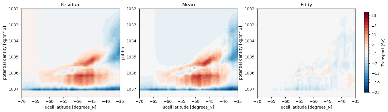
This method results in a smoother vertical distribution than xhistogram, as it is not quite a histogram but does some interpolation to the top and bottom of each vertical cell. We have found that the computation currently has issues with interior land boundaries: xgcm isn’t able to compute partial cells at the bottom of the ocean in MOM5. We thus add a correction after the computation to ensure that vertical integrals are preserved and thus that streamfunctions calculated are closed.

Load vertical grid bin centres and edges¶

[15]:

%%time

ds = expt_datastore.search(
    variable=['st_ocean','st_edges_ocean'],
    frequency='1mon', # and `frequency` gets us down to a single dataset
    start_date='2170-0[1-3].*',
).to_dask(
    xarray_open_kwargs={
        'chunks' : 'auto', # This is the easiest way to get a dataset to open relatively quickly
    }
)

st_ocean = ds['st_ocean']
st_edges_ocean = ds['st_edges_ocean']

CPU times: user 4.04 s, sys: 1.13 s, total: 5.17 s
Wall time: 6.75 s

Define edge of target density bins¶

[16]:

ds = expt_datastore.search(
    variable='potrho_edges',
    frequency='1mon',
    start_date='2170-0[1-3].*',
).to_dask(
    xarray_open_kwargs={
        'chunks' : 'auto', # This is the easiest way to get a dataset to open relatively quickly
    }
)


pot_rho_2_target = ds['potrho_edges'].values

Calculate vertical regridding into density coordinates¶

[17]:

%%time

ds = xr.Dataset({'ty_trans': ty_trans, 'pot_rho_2': pot_rho_2})

# Note: Quantity must be extensive, e.g., ty_trans, vhrho_nt, uhrho_et, tx_trans but *not*, e.g., v, salt.
#       If not extensive, then we need to multiply by dzt or dzu.
ds = ds.assign_coords({'st_edges_ocean': st_edges_ocean})
ds = ds.chunk({'st_edges_ocean': 76, 'st_ocean': 75}) # xgcm doesn't like it if there is more than 1 chunk in this axis

grid = xgcm.Grid(ds, coords={'Z': {'center': 'st_ocean', 'outer': 'st_edges_ocean'}}, periodic = False)
ds['pot_rho_2_outer'] = grid.interp(ds.pot_rho_2, 'Z', boundary='extend')
ds['pot_rho_2_outer'] = ds['pot_rho_2_outer'].chunk({'st_edges_ocean': 76})

ty_trans_transformed_cons = grid.transform(ds.ty_trans,
                                           'Z',
                                           pot_rho_2_target,
                                           method='conservative',
                                           target_data=ds.pot_rho_2_outer)

### change name to fit previous bins because default xgcm naming is different
# pot_rho_2_outer is actually the CENTRE of bins (I guess the convention was defined for linear interpolation not conservative)
ty_trans_transformed_cons = ty_trans_transformed_cons.rename({'pot_rho_2_outer': 'potrho'})

CPU times: user 33.1 ms, sys: 0 ns, total: 33.1 ms
Wall time: 31.4 ms

[18]:

%%time
ty_trans_transformed_cons = ty_trans_transformed_cons.load()

CPU times: user 3.79 s, sys: 1.74 s, total: 5.53 s
Wall time: 7.8 s

Now account for partial cell at bottom¶

We do this by finding what is missing from the vertical integral (residual). This is what was in the partial cell. We then add that residual into the densest cell that currently exists in the transformed data. This is only an approximation, because the density of the partial cell may be denser than that of the cell above it. However, this correction means the vertical integral is preserved under the transformation.

[19]:

%%time
#find residual from vertical integral
ty_trans_residual = ty_trans.sum('st_ocean') - ty_trans_transformed_cons.sum('potrho') #this is positive definite

CPU times: user 1.25 s, sys: 661 ms, total: 1.91 s
Wall time: 1.28 s

Find bottom density of `ty_trans_transformed_cons`¶

[20]:

%%time
# select out bottom values:
ty_trans_transformed_cons2 = ty_trans_transformed_cons.where(ty_trans_transformed_cons != 0)
dens_array = ty_trans_transformed_cons2 * 0 + ty_trans_transformed_cons2.potrho # array of isopycnal value where it exists and nan elsewhere
max_dens = dens_array.max(dim = 'potrho', skipna = True)

CPU times: user 1.68 s, sys: 970 ms, total: 2.65 s
Wall time: 1.77 s

Add residual to this bottom density in array¶

[21]:

%%time
ty_trans_residual_array = (dens_array.where(dens_array == max_dens)*0 + 1) * ty_trans_residual
ty_trans_new = ty_trans_residual_array.fillna(0)+ ty_trans_transformed_cons

CPU times: user 2.86 s, sys: 1.54 s, total: 4.39 s
Wall time: 2.92 s

[22]:

# rename coords to match ty_trans_rho
ty_trans_new = ty_trans_new.rename({'yu_ocean': 'grid_yu_ocean', 'xt_ocean': 'grid_xt_ocean'})

[ ]:

%%time
# We need to rechunk here to make the chunks a bit smaller, otherwise the dask workers will die.
# I've halved the chunk size on `grid_xt_ocean` and `potrho`. Sometimes, {'chunks' : 'auto'} can be
# a bit too ambitious!

ty_trans_new = ty_trans_new.chunk(
    chunks = {
        'grid_yu_ocean': 337,
        'grid_xt_ocean': 200, # was 400
        'potrho': 40, # was 80
    }
)
ty_trans_new = ty_trans_new.load()

Plot streamfunction of result¶

[24]:

psi_avg_mean_2 = cumsum_from_bottom(ty_trans_new.sum('grid_xt_ocean') / (1e6 * rho_0))

[25]:

%%time

fig, axes = plt.subplots(nrows = 1, ncols = 3, figsize = (15, 4))

levels = np.linspace(-25, 25, 26)

psi_avg.plot.contourf(ax = axes[0], x = 'grid_yu_ocean',levels = levels, add_colorbar = False)

psi_avg_mean_2.plot.contourf(ax = axes[1], x = 'grid_yu_ocean', levels = levels, add_colorbar = False)

p = (psi_avg - psi_avg_mean_2).plot.contourf(ax = axes[2], x = 'grid_yu_ocean', levels = levels, add_colorbar = False)

cbar_ax = fig.add_axes([0.92, 0.15, 0.01, 0.7])
fig.colorbar(p, cax=cbar_ax, label='Transport (Sv)')

axes[0].set_title('Residual')
axes[1].set_title('Mean')
axes[2].set_title('Eddy')

for ax in axes:
    ax.set_ylim(1037.5, 1032)
    ax.set_xlim(-70, -35);

2025-08-14 14:54:45,788 - distributed.worker.memory - WARNING - Unmanaged memory use is high. This may indicate a memory leak or the memory may not be released to the OS; see https://distributed.dask.org/en/latest/worker-memory.html#memory-not-released-back-to-the-os for more information. -- Unmanaged memory: 2.63 GiB -- Worker memory limit: 3.93 GiB

CPU times: user 10.1 s, sys: 5.92 s, total: 16 s
Wall time: 22.7 s

../_images/03-Advanced-Recipes_Transformation_from_Depth_to_Potential_Density_39_2.png

Method 3: Bin `ty_trans` (mean Eulerian overturning) into density bins¶

This uses the method by Lee et al. (2007) and which is is described as follows. Firstly, cells in the model output with a density \(\rho\) between two prescribed densities (\(\rho_\text{heavy} >\rho> \rho_\text{light}\)) are selected. Each cell is assigned a proximity to the lighter density \(\rho_\text{light}\), which is the ‘bin fraction’

\[f_b = \frac{\rho_\text{heavy}-\rho}{\rho_\text{heavy}-\rho_\text{light}}.\]

Here, a bin fraction of 1 means the cell density \(\rho = \rho_\text{light}\) and \(f_b=0\) means \(\rho = \rho_\text{heavy}\). The quantity being binned, such as the meridional transport \(vh\), is then multiplied by \(f_b\) and added to the lighter density \(\rho_\text{light}\) bin’s meridional transport, followed by the \(vh(1-f_b)\) being added to the heavier bin, \(\rho_\text{heavy}\). This process is repeated for all sets of consecutive bins, meaning that density bins have input from model output cells with density slightly lower and higher than it.

Lee, M., Nurser, A., Coward, A., and De Cuevas, B. (2007). Eddy advective and diffusive transports of heat and salt in the Southern Ocean. Journal of Physical Oceanography, 37(5), 1376–1393.

For this method, we need to get rid of NaNs¶

[26]:

ty_trans = ty_trans.fillna(0)
pot_rho_2 = pot_rho_2.fillna(0)

Load first to reduce computation time¶

[27]:

%%time
pot_rho_2 = pot_rho_2.load()
ty_trans = ty_trans.load()

CPU times: user 6.25 s, sys: 3.05 s, total: 9.3 s
Wall time: 13.6 s

[28]:

# choose bins (in this case, default ty_trans_rho pot_rho_2 bins
rho2_bins = ty_trans_rho.potrho.values

# set up a zero array to be filled in by the algorithm
ty_trans_binned = np.zeros((len(rho2_bins), len(pot_rho_2.yu_ocean), len(pot_rho_2.xt_ocean)))

Note: the following cell takes a while.

[29]:

%%time

from tqdm.auto import tqdm

# loop over the bins, performing algorithm by Lee et al. (2007)
# note that it takes time; faster if ty_trans and pot_rho_2 already loaded
for i in tqdm(range(len(rho2_bins)-1)):
    bin_mask = pot_rho_2.where(pot_rho_2 <= rho2_bins[i+1]).where(pot_rho_2 > rho2_bins[i])*0 + 1
    bin_fractions = (rho2_bins[i+1] - pot_rho_2 * bin_mask) / (rho2_bins[i+1] - rho2_bins[i])
    ## bin ty_trans:
    ty_trans_in_lower_bin = (ty_trans * bin_mask * bin_fractions).sum(dim = 'st_ocean')
    ty_trans_binned[i, :, :] += ty_trans_in_lower_bin.fillna(0).values
    del ty_trans_in_lower_bin
    ty_trans_in_upper_bin = (ty_trans * bin_mask * (1 - bin_fractions)).sum(dim = 'st_ocean')
    ty_trans_binned[i+1, :, :] += ty_trans_in_upper_bin.fillna(0).values
    del ty_trans_in_upper_bin

CPU times: user 10min 15s, sys: 7min 45s, total: 18min
Wall time: 11min 55s

[30]:

# convert numpy array into xarray dataarray
ty_trans_binned_array = xr.DataArray(ty_trans_binned,
                                     coords = [rho2_bins, pot_rho_2.yu_ocean, pot_rho_2.xt_ocean],
                                     dims = ['potrho', 'grid_yu_ocean', 'grid_xt_ocean'],
                                     name = 'ty_trans_binned')

[31]:

# find streamfunction
psi_avg_mean_3 = cumsum_from_bottom(ty_trans_binned_array.sum('grid_xt_ocean')) / (1e6 * rho_0)

Plot streamfunctions¶

[32]:

fig, axes = plt.subplots(nrows = 1, ncols = 3, figsize = (15, 4))

levels = np.linspace(-25, 25, 26)

psi_avg.plot.contourf(ax = axes[0], x = 'grid_yu_ocean',levels = levels, add_colorbar = False)

psi_avg_mean_3.plot.contourf(ax = axes[1], x = 'grid_yu_ocean', levels = levels, add_colorbar = False)

p = (psi_avg - psi_avg_mean_3).plot.contourf(ax = axes[2], x = 'grid_yu_ocean', levels = levels, add_colorbar = False)

cbar_ax = fig.add_axes([0.92, 0.15, 0.01, 0.7])
fig.colorbar(p, cax = cbar_ax, label = 'Transport (Sv)')

axes[0].set_title('Residual')
axes[1].set_title('Mean')
axes[2].set_title('Eddy')

for ax in axes:
    ax.set_ylim(1037.5, 1032)
    ax.set_xlim(-70, -35);

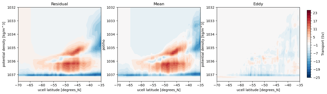
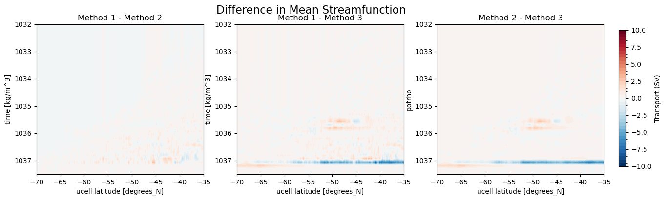
../_images/03-Advanced-Recipes_Transformation_from_Depth_to_Potential_Density_51_0.png

All three methods yield similar plots of the decomposition of the meridional overturning streamfunction.¶

The exact numbers resulting from the transformations differ, due to the different numerical methods. xhistogram is exact when compared to snapshots of MOM5 model output, and is hence most appropriate when comparing between online and offline binned quantities. xgcm and the Lee method can still be used to compare quantities binned offline. For example, if we were to instead bin the daily transports onto isopycnals and calculate eddy terms directly from the correlation of velocity and thickness fluctuations, xgcm and the Lee method may be better as the weighted binning onto isopycnals leaves less chance of ‘gaps’ between density layers. The Lee method has no issues with partial cells, but it is much slower than xgcm.

The difference in the mean streamfunction between the three methods is presented below.

[33]:

fig, axes = plt.subplots(nrows = 1, ncols = 3, figsize = (15, 4))

levels = np.arange(-10, 10.1, 0.5)

(psi_avg_mean - psi_avg_mean_2).plot.contourf(ax = axes[0], x = 'grid_yu_ocean',levels = levels, add_colorbar = False)

(psi_avg_mean - psi_avg_mean_3).plot.contourf(ax = axes[1], x = 'grid_yu_ocean', levels = levels, add_colorbar = False)

p = (psi_avg_mean_2 - psi_avg_mean_3).plot.contourf(ax = axes[2], x = 'grid_yu_ocean', levels = levels, add_colorbar = False)

cbar_ax = fig.add_axes([0.92, 0.15, 0.01, 0.7])
fig.colorbar(p, cax=cbar_ax, label='Transport (Sv)')

axes[0].set_title('Method 1 - Method 2')
axes[1].set_title('Method 1 - Method 3')
axes[2].set_title('Method 2 - Method 3')

for ax in axes:
    ax.set_ylim(1037.5, 1032)
    ax.set_xlim(-70, -35)

fig.suptitle('Difference in Mean Streamfunction', fontsize = 16);

2025-08-14 15:07:34,392 - distributed.worker.memory - WARNING - Unmanaged memory use is high. This may indicate a memory leak or the memory may not be released to the OS; see https://distributed.dask.org/en/latest/worker-memory.html#memory-not-released-back-to-the-os for more information. -- Unmanaged memory: 2.72 GiB -- Worker memory limit: 3.93 GiB

../_images/03-Advanced-Recipes_Transformation_from_Depth_to_Potential_Density_53_1.png

An alternative method to calculate the decomposition of the residual meridional overturning circulation into mean and eddy components is to bin ty_trans (or vhrho_nt) into density bins using daily data (both density and transport). Then the transport \(\overline{vh}\) can be separated into a mean component \(\overline{v}\overline{h}\) and an eddy component \(\overline{v^\prime h^\prime}\), where the overline is a time average and primed quantities the deviation from the time average. Quantities are calculated within density layers, and \(h\) is density layer thickness, calculated by binning dzt or dzu. This calculation, since it uses daily data, is computationally expensive and is difficult to do efficiently in a Jupyter notebook. The resulting streamfunctions are similar, but not identical, and may be more intuitive for isopycnal flows. An example of this method can be found at https://github.com/claireyung/Topographic_Hotspots_Upwelling-Paper_Code/blob/main/Figure_Code/Fig5-Overturning.ipynb.