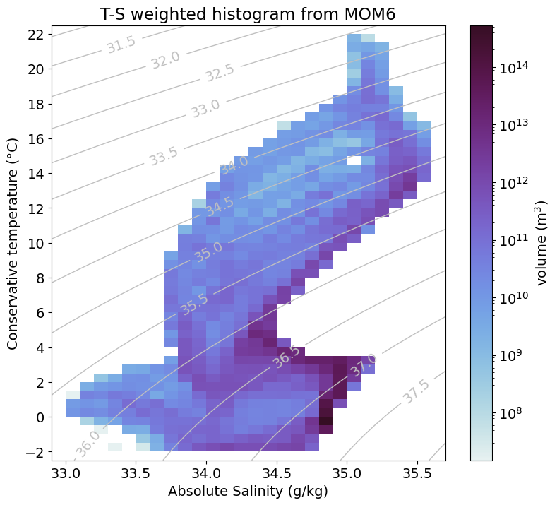
This notebook shows how to plot a temperature-salinity diagram which is weighted by volume using xhistogram.
The notebook is written using output from MOM6. If you want to use output from MOM5 the relevant diagnostics are as follows;
Temperature: temp which is conservative temperature (in MOM6 we use potential temperature thetao)
Salinity: salt (in MOM6 this is so)
In MOM6, there is a tracer cell volume diagnostic (volcello). There is no output diagnostic equivalent in MOM5, however you can calculate the tracer cell volume by multiplying the tracer cell area (area_t) by the tracer cell thickness (dzt).
Note that the coordinate (lat and lon) names also differ between MOM6 and MOM5. In MOM6, the tracer longitude coordinate is labelled xh, the tracer latitude coordinate is labelled yh, and the tracer vertical coordinate is z_l. In MOM5, the tracer longitude coordinate is labelled xt_ocean, the tracer latitude coordinate is labelled yt_ocean, and the tracer vertical coordinate is st_ocean.
Requirements: The conda/analysis3 (or later) module on ARE. A session with 4 cores is sufficient for this example but more cores will be needed for larger datasets.
Firstly, we load all required modules and start a client.
[1]:
# analysis librariesimportxarrayasxrimportnumpyasnpimportgswfromxhistogram.xarrayimporthistogramasxhistogram# intake and Daskimportintakecatalog=intake.cat.access_nrifromdask.distributedimportClient# plotting libariesimportmatplotlib.pyplotaspltimportcmocean.cmascmoimportmatplotlib.colorsascolors
Choose an experiment of any resolution. Here, only 1 year of the MOM6 panant-01-zstar-v13 experiment is selected; if you want to use a longer time period, you might need more resources!
We define a function below to load output (temperature or salinity) on which we will compute the histogram for the T-S diagram.
[4]:
defload_data(variable,frequency='1mon',file_id=None,start_time=None,end_time=None):''' variable: string defining the variable to load (e.g. `thetao` or `so`) '''catalog_subset=catalog[experiment]variable_search=catalog_subset.search(variable=variable,frequency=frequency)iffile_idisnotNone:variable_search=variable_search.search(file_id=file_id)darray=variable_search.to_dask(xarray_open_kwargs={"decode_timedelta":False})darray=darray.get(variable)if'time'indarray.coords:darray=darray.sel(time=slice(start_time,end_time))returndarray
Now we need to convert from potential temperature to conservative temperature and from practical salinity to absolute salinity. If adapting this to MOM5 output, make sure you check the temperature and salinity definitions/units - they may be different than for MOM6! To learn more about the different types of salinity and temperature measurements, and how to convert between them, visit the GSW toolbox: https://teos-10.github.io/GSW-Python/intro.html
[8]:
# Calculate ocean pressure (gsw assumes ocean depth is positive upwards,# hence the negative applied here)pressure=gsw.p_from_z(-salt.z_l,salt.yh)# This converts pratical salinity (psu) to absolute salinity (g/kg)SA=gsw.SA_from_SP(salt,pressure,salt.xh,salt.yh)SA.attrs={'units':'Absolute Salinity (g/kg)'}# This converts potential temperature (deg C) to conservative temperature (deg C)CT=gsw.CT_from_pt(salt,temperature)CT=CT.rename('thetao')CT.attrs={'units':'Conservative temperature (°C)'}
Now load the converted data into memory. Note: You don’t need to load the data into memory to run the rest of the script but it can make subsequent calculations faster. However, if you choose to load more data (e.g. a larger region or longer timeframe) then this step might cause the kernel to die.
Now define the function that computes the temperature and salinity bins for the T-S histogram.
[10]:
defcompute_TS_bins(salt,temperature,volume):temp_bins=np.arange(np.floor(temperature.min().values)-0.5,np.ceil(temperature.max().values)+0.6,0.5)salt_bins=np.arange(np.floor(salt.min().values)-0.1,np.ceil(salt.max().values)+0.11,0.1)# To create density contours in the T-S diagramtemp_bins_mesh,salt_bins_mesh=np.meshgrid(temp_bins,salt_bins)TS_density=gsw.density.sigma2(salt_bins_mesh,temp_bins_mesh)# Create the 2D histogram array containing the temperature and salinity values,# weighted by grid cell volumeTS_histogram=xhistogram(temperature,salt,bins=(temp_bins,salt_bins),weights=volume)TS_histogram=TS_histogram.where(TS_histogram!=0).compute()returnTS_histogram,TS_density,salt_bins_mesh,temp_bins_mesh
/g/data/xp65/public/apps/med_conda/envs/analysis3-26.06/lib/python3.12/site-packages/distributed/client.py:3387: UserWarning: Sending large graph of size 13.02 MiB.
This may cause some slowdown.
Consider loading the data with Dask directly
 or using futures or delayed objects to embed the data into the graph without repetition.
See also https://docs.dask.org/en/stable/best-practices.html#load-data-with-dask for more information.
  warnings.warn(
CPU times: user 2.72 s, sys: 1.49 s, total: 4.22 s
Wall time: 3.93 s
plt.rcParams['font.size']=14plt.figure(figsize=(9,8))# normalize the colorbar to the min and maximum values of the histogram# using a LogNormal scalenorm=colors.LogNorm(vmin=TS_histogram.min().values,vmax=TS_histogram.max().values)# Plot (shade) the TS histogram dataTS_histogram.plot(cmap=cmo.dense,norm=norm,cbar_kwargs=dict(label='volume (m$^{3}$)'))# Add the density contourscs=plt.contour(salt_bins_mesh,temp_bins_mesh,TS_density,colors='silver',linewidths=1,levels=np.arange(np.floor(TS_density.min()),np.ceil(TS_density.max()),.5))plt.clabel(cs,inline=True)plt.xlabel(SA.units)plt.ylabel(CT.units)plt.title("T-S weighted histogram from MOM6");plt.xlim([32.9,35.7])plt.yticks(np.arange(-2,23,2))plt.show()