In MOM5 velocities are calculated in the (north-east) corner of the cells, where the dimension names are xu_ocean and yu_ocean. In MOM6, velocities are calculated in the eastern face of the cell for uo and northern face of the cell for vo. To adapt this recipe, an option would be to interpolate first uo and vo to be in the (north-east) corner, where the dimensions are (xq, yq). For more information on grids and xgcm, refer to [INSERT UPCOMING TUTORIAL ON
GRIDS].
There are a few different options for the zonal and meridional lengths of the cells as well, which you can use depending on how you perform the xgcm interpolation and differentiation.
Load model variables needed. We will only load one month of daily data, and we will select a subset over a Subantarctic Front meander in the Antarctic Circumpolar Current.
/g/data/xp65/public/apps/med_conda/envs/analysis3-25.09/lib/python3.11/site-packages/intake_esm/core.py:321: FutureWarning: When grouping with a length-1 list-like, you will need to pass a length-1 tuple to get_group in a future version of pandas. Pass `(name,)` instead of `name` to silence this warning.
  records = grouped.get_group(internal_key).to_dict(orient='records')
Load grid coordinates and sizes.
[46]:
# Load coordinates and grid specificationsdarray=cat_subset.search(variable=['dxu'],frequency='fx').to_dask()dxu=darray['dxu'].sel(xu_ocean=slice(-224.2,-212.0),yu_ocean=slice(-53.5,-47.5))darray=cat_subset.search(variable=['dyu'],frequency='fx').to_dask()dyu=darray['dyu'].sel(xu_ocean=slice(-224.2,-212.0),yu_ocean=slice(-53.5,-47.5))
/g/data/xp65/public/apps/med_conda/envs/analysis3-25.09/lib/python3.11/site-packages/intake_esm/core.py:321: FutureWarning: When grouping with a length-1 list-like, you will need to pass a length-1 tuple to get_group in a future version of pandas. Pass `(name,)` instead of `name` to silence this warning.
  records = grouped.get_group(internal_key).to_dict(orient='records')
/g/data/xp65/public/apps/med_conda/envs/analysis3-25.09/lib/python3.11/site-packages/intake_esm/source.py:308: ConcatenationWarning: Attempting to concatenate datasets without valid dimension coordinates: retaining only first dataset. Request valid dimension coordinate to silence this warning.
  warnings.warn(
The way xgcm works is that we first create a grid object that has all the information regarding our staggered grid. For our case, grid needs to know the location of the xt_ocean, xu_ocean points (and same for y) and their relative orientation to one another, i.e., that xu_ocean is shifted to the right of xt_ocean by \(\frac{1}{2}\) grid-cell.
<xgcm.Grid>
Y Axis (not periodic, boundary='extend'):
  * center   yt_ocean --> inner
  * inner    yu_ocean --> center
X Axis (not periodic, boundary='extend'):
  * center   xt_ocean --> right
  * right    xu_ocean --> center
The geostrophic velocities at the surface can be calculated from sea level contours. This can be done from satellite altimetry by using the SSH contours or in the ACCESS-OM2 simulation by using the sea level contours. The relation between the surface geostrophic zonal (\(u_{g,s}\)) and meridional (\(v_{g,s}\)) velocities and the sea level (\(\eta\)) are as follow:
Now, we just have to provide the function geostrophic_velocity with the variables in the Dataset, the Grid made with xgcm, we set stream_func to None, because we only calculate the geostrophic velocities at the surface and we provide the names of \(dx\) and \(dy\) in the Dataset.
[50]:
# calculating the geostrophic flow speedVg=np.sqrt(ds['ug_s']**2+ds['vg_s']**2)
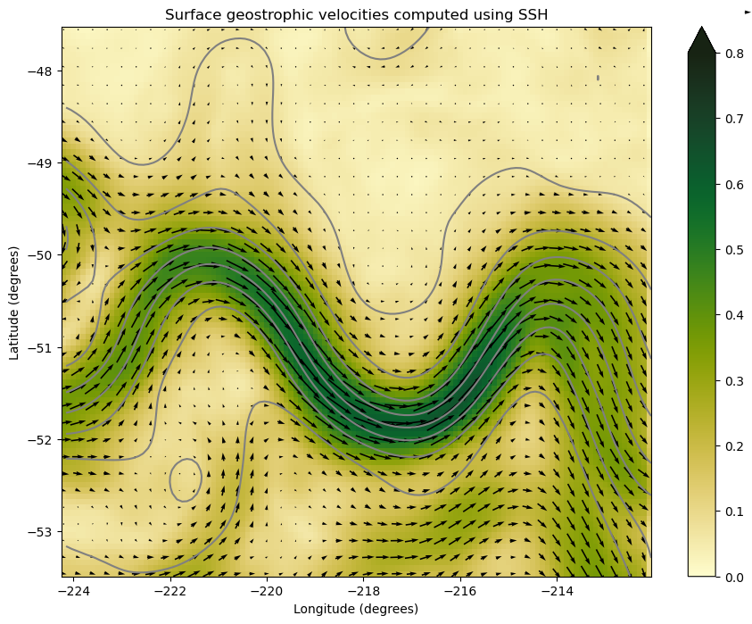
We have now calculated the geostrophic velocities and we can make a plot, in which we show the geostrophic flow speed averaged over the 16-day period with the sea level contours overlaid.
[53]:
# to select every third cellslc=xt_ocean=slice(None,None,3)Vg.mean('time').plot(size=8,cmap=cm.cm.speed,vmin=0,vmax=0.8,extend='max')ds['sea_level'].mean('time').plot.contour(levels=np.linspace(-0.7,0,8),colors='gray',linestyles='solid')ds.mean('time').sel(xu_ocean=slc,yu_ocean=slc).plot.quiver(x='xu_ocean',y='yu_ocean',u='ug_s',v='vg_s')plt.xlabel('Longitude (degrees)')plt.ylabel('Latitude (degrees)')plt.title('Surface geostrophic velocities computed using SSH');
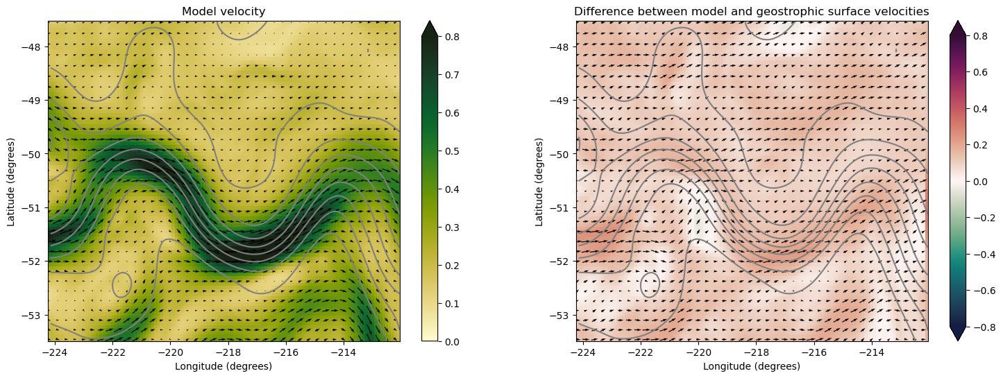
We can compare the geostrophic velocities to the total simulated velocities at the surface and see what the difference in flow speed is. The difference is made up of the various contributions to the ageostrophic flow, such as the Ekman velocities and velocities driven by advection (curvature in the flow field).
[54]:
# calculating the total flow speed from the simulated velocities at the surfaceV_s=np.sqrt(ds['u']**2+ds['v']**2)ds['uag']=ds['u']-ds['ug_s']ds['vag']=ds['v']-ds['vg_s']
[56]:
fig,axes=plt.subplots(nrows=1,ncols=2,figsize=(18,6))# Plot total flow speedV_s.mean('time').plot(ax=axes[0],cmap=cm.cm.speed,vmin=0,vmax=0.8)ds.mean('time').sel(xu_ocean=slc,yu_ocean=slc).plot.quiver(ax=axes[0],x='xu_ocean',y='yu_ocean',u='u',v='v',add_guide=False)# Plot ageostrophic flow speed(V_s-Vg).mean('time').plot(ax=axes[1],cmap=cm.cm.curl,vmin=-0.8,vmax=0.8,extend='both')ds.mean('time').sel(xu_ocean=slc,yu_ocean=slc).plot.quiver(ax=axes[1],x='xu_ocean',y='yu_ocean',u='uag',v='vag',add_guide=False)foraxinaxes:ds['sea_level'].mean('time').plot.contour(ax=ax,levels=np.linspace(-0.7,0,8),colors='gray',linestyles='solid')ax.set_xlabel('Longitude (degrees)')ax.set_ylabel('Latitude (degrees)')axes[0].set_title('Model velocity')axes[1].set_title('Difference between model and geostrophic surface velocities');
It is interesting that the total flow speed is almost everywhere larger than the geostrophic flow speed due to the prevailing westerlies. However, where the streamlines are strongly curved agesotrophic velocities due to the advection (curvature) terms become important.