Kinetic Energy Mean-Transient Decomposition
Decomposing the kinetic energy into time-mean and transient components.
Theory
For a hydrostatic ocean model, like MOM5, the relevant kinetic energy per unit mass is
The vertical velocity component, \(w\), does not appear in the mechanical energy budget. It is very much subdominant. But more fundamentally, it simply does not appear in the mechanical energy buget for a hydrostatic ocean.
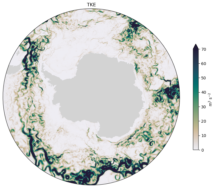
For a non-steady fluid, we can define the time-averaged kinetic energy as the total kinetic energy, TKE
It is useful to decompose the velocity into time-mean and time-varying components, e.g.,
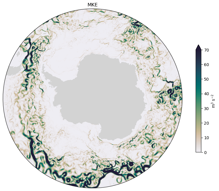
The mean kinetic energy is the energy associated with the mean flow
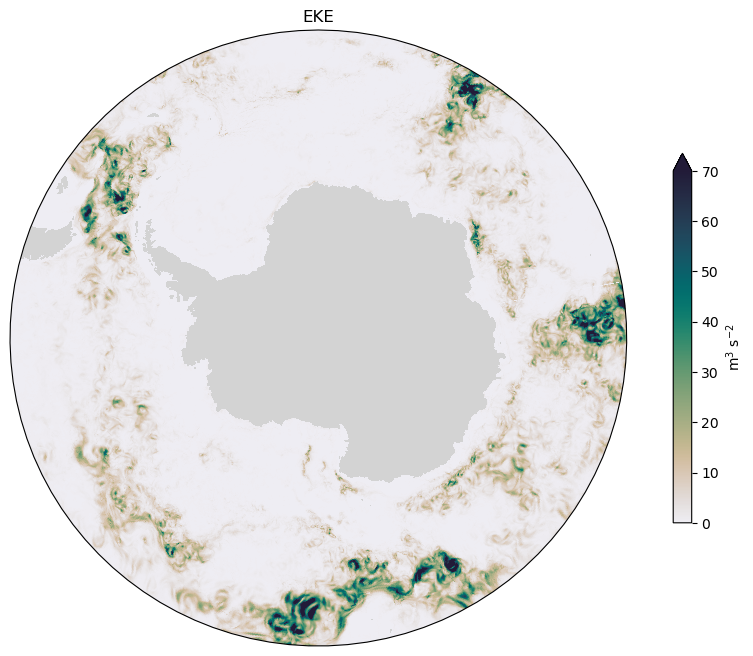
The kinetic energy of the time varying component is the eddy kinetic energy, EKE. This quantity can be obtained by substracting the velocity means and calculating the kinetic energy of the perturbation velocity quantities.
MKE and EKE partition the total kinetic energy
Adapting for MOM6
Variable |
MOM5 diagnostic |
Equivalent MOM6 diagnostic |
|---|---|---|
Zonal velocity (m/s) |
|
|
Meridional velocity (m/s) |
|
|
Cell thickness (m) |
|
Not available for most experiments, but can be calculated by |
In MOM5 velocities are calculated in the (north-east) corner of the cells, where the dimension names are xu_ocean and yu_ocean. In MOM6, velocities are calculated in the eastern face of the cell for uo and northern face of the cell for vo. To adapt this recipe, an option would be to interpolate first uo and vo to be in the (north-east) corner, where the dimensions are (xq, yq).
MOM5
We start by importing some useful packages.
[1]:
import cartopy.crs as ccrs
import cartopy.feature as feature
import cmocean as cm
import intake
import matplotlib.path as mpath
import matplotlib.pyplot as plt
import numpy as np
import xarray as xr

from dask.distributed import Client
[2]:
client = Client(threads_per_worker = 1)
client
[2]:
Client
Client-872d97b8-49a5-11f1-8b38-000003b1fe80
| Connection method: Cluster object | Cluster type: distributed.LocalCluster |
| Dashboard: /proxy/8787/status |
Cluster Info
LocalCluster
6508c3fc
| Dashboard: /proxy/8787/status | Workers: 28 |
| Total threads: 28 | Total memory: 125.19 GiB |
| Status: running | Using processes: True |
Scheduler Info
Scheduler
Scheduler-171cd5e2-68d8-4775-8477-5ee670f6c579
| Comm: tcp://127.0.0.1:33179 | Workers: 0 |
| Dashboard: /proxy/8787/status | Total threads: 0 |
| Started: Just now | Total memory: 0 B |
Workers
Worker: 0
| Comm: tcp://127.0.0.1:37993 | Total threads: 1 |
| Dashboard: /proxy/33639/status | Memory: 4.47 GiB |
| Nanny: tcp://127.0.0.1:40409 | |
| Local directory: /jobfs/167820005.gadi-pbs/dask-scratch-space/worker-_xjhqdem | |
Worker: 1
| Comm: tcp://127.0.0.1:36809 | Total threads: 1 |
| Dashboard: /proxy/42025/status | Memory: 4.47 GiB |
| Nanny: tcp://127.0.0.1:46407 | |
| Local directory: /jobfs/167820005.gadi-pbs/dask-scratch-space/worker-91lpopg0 | |
Worker: 2
| Comm: tcp://127.0.0.1:37735 | Total threads: 1 |
| Dashboard: /proxy/40133/status | Memory: 4.47 GiB |
| Nanny: tcp://127.0.0.1:42631 | |
| Local directory: /jobfs/167820005.gadi-pbs/dask-scratch-space/worker-csrp1krt | |
Worker: 3
| Comm: tcp://127.0.0.1:39459 | Total threads: 1 |
| Dashboard: /proxy/32777/status | Memory: 4.47 GiB |
| Nanny: tcp://127.0.0.1:42105 | |
| Local directory: /jobfs/167820005.gadi-pbs/dask-scratch-space/worker-rigraf8h | |
Worker: 4
| Comm: tcp://127.0.0.1:33883 | Total threads: 1 |
| Dashboard: /proxy/35353/status | Memory: 4.47 GiB |
| Nanny: tcp://127.0.0.1:44111 | |
| Local directory: /jobfs/167820005.gadi-pbs/dask-scratch-space/worker-lat57oeg | |
Worker: 5
| Comm: tcp://127.0.0.1:41927 | Total threads: 1 |
| Dashboard: /proxy/45887/status | Memory: 4.47 GiB |
| Nanny: tcp://127.0.0.1:34367 | |
| Local directory: /jobfs/167820005.gadi-pbs/dask-scratch-space/worker-og5bdwgm | |
Worker: 6
| Comm: tcp://127.0.0.1:36391 | Total threads: 1 |
| Dashboard: /proxy/45509/status | Memory: 4.47 GiB |
| Nanny: tcp://127.0.0.1:32987 | |
| Local directory: /jobfs/167820005.gadi-pbs/dask-scratch-space/worker-xt0x9q92 | |
Worker: 7
| Comm: tcp://127.0.0.1:43543 | Total threads: 1 |
| Dashboard: /proxy/36503/status | Memory: 4.47 GiB |
| Nanny: tcp://127.0.0.1:43495 | |
| Local directory: /jobfs/167820005.gadi-pbs/dask-scratch-space/worker-1oqahwjl | |
Worker: 8
| Comm: tcp://127.0.0.1:35393 | Total threads: 1 |
| Dashboard: /proxy/33503/status | Memory: 4.47 GiB |
| Nanny: tcp://127.0.0.1:39601 | |
| Local directory: /jobfs/167820005.gadi-pbs/dask-scratch-space/worker-_romjcz5 | |
Worker: 9
| Comm: tcp://127.0.0.1:33861 | Total threads: 1 |
| Dashboard: /proxy/43517/status | Memory: 4.47 GiB |
| Nanny: tcp://127.0.0.1:40097 | |
| Local directory: /jobfs/167820005.gadi-pbs/dask-scratch-space/worker-eligom4s | |
Worker: 10
| Comm: tcp://127.0.0.1:34035 | Total threads: 1 |
| Dashboard: /proxy/43923/status | Memory: 4.47 GiB |
| Nanny: tcp://127.0.0.1:43589 | |
| Local directory: /jobfs/167820005.gadi-pbs/dask-scratch-space/worker-vpmw3hqy | |
Worker: 11
| Comm: tcp://127.0.0.1:36737 | Total threads: 1 |
| Dashboard: /proxy/43153/status | Memory: 4.47 GiB |
| Nanny: tcp://127.0.0.1:33725 | |
| Local directory: /jobfs/167820005.gadi-pbs/dask-scratch-space/worker-0ls8row2 | |
Worker: 12
| Comm: tcp://127.0.0.1:35667 | Total threads: 1 |
| Dashboard: /proxy/41623/status | Memory: 4.47 GiB |
| Nanny: tcp://127.0.0.1:45993 | |
| Local directory: /jobfs/167820005.gadi-pbs/dask-scratch-space/worker-p7kvfc7p | |
Worker: 13
| Comm: tcp://127.0.0.1:34213 | Total threads: 1 |
| Dashboard: /proxy/43389/status | Memory: 4.47 GiB |
| Nanny: tcp://127.0.0.1:33901 | |
| Local directory: /jobfs/167820005.gadi-pbs/dask-scratch-space/worker-25_s20mn | |
Worker: 14
| Comm: tcp://127.0.0.1:43975 | Total threads: 1 |
| Dashboard: /proxy/36433/status | Memory: 4.47 GiB |
| Nanny: tcp://127.0.0.1:39009 | |
| Local directory: /jobfs/167820005.gadi-pbs/dask-scratch-space/worker-megx07ht | |
Worker: 15
| Comm: tcp://127.0.0.1:34347 | Total threads: 1 |
| Dashboard: /proxy/43387/status | Memory: 4.47 GiB |
| Nanny: tcp://127.0.0.1:39507 | |
| Local directory: /jobfs/167820005.gadi-pbs/dask-scratch-space/worker-80jij21t | |
Worker: 16
| Comm: tcp://127.0.0.1:37779 | Total threads: 1 |
| Dashboard: /proxy/42727/status | Memory: 4.47 GiB |
| Nanny: tcp://127.0.0.1:36585 | |
| Local directory: /jobfs/167820005.gadi-pbs/dask-scratch-space/worker-sxk7vr_f | |
Worker: 17
| Comm: tcp://127.0.0.1:45673 | Total threads: 1 |
| Dashboard: /proxy/33437/status | Memory: 4.47 GiB |
| Nanny: tcp://127.0.0.1:36425 | |
| Local directory: /jobfs/167820005.gadi-pbs/dask-scratch-space/worker-oh_zfsav | |
Worker: 18
| Comm: tcp://127.0.0.1:33773 | Total threads: 1 |
| Dashboard: /proxy/33993/status | Memory: 4.47 GiB |
| Nanny: tcp://127.0.0.1:46693 | |
| Local directory: /jobfs/167820005.gadi-pbs/dask-scratch-space/worker-518h3tkj | |
Worker: 19
| Comm: tcp://127.0.0.1:42847 | Total threads: 1 |
| Dashboard: /proxy/37149/status | Memory: 4.47 GiB |
| Nanny: tcp://127.0.0.1:36411 | |
| Local directory: /jobfs/167820005.gadi-pbs/dask-scratch-space/worker-bjqyo3jl | |
Worker: 20
| Comm: tcp://127.0.0.1:34735 | Total threads: 1 |
| Dashboard: /proxy/46483/status | Memory: 4.47 GiB |
| Nanny: tcp://127.0.0.1:39415 | |
| Local directory: /jobfs/167820005.gadi-pbs/dask-scratch-space/worker-hvbrygl7 | |
Worker: 21
| Comm: tcp://127.0.0.1:45889 | Total threads: 1 |
| Dashboard: /proxy/40985/status | Memory: 4.47 GiB |
| Nanny: tcp://127.0.0.1:35609 | |
| Local directory: /jobfs/167820005.gadi-pbs/dask-scratch-space/worker-ud8_s_cq | |
Worker: 22
| Comm: tcp://127.0.0.1:44211 | Total threads: 1 |
| Dashboard: /proxy/35329/status | Memory: 4.47 GiB |
| Nanny: tcp://127.0.0.1:34385 | |
| Local directory: /jobfs/167820005.gadi-pbs/dask-scratch-space/worker-a_g8pte6 | |
Worker: 23
| Comm: tcp://127.0.0.1:34839 | Total threads: 1 |
| Dashboard: /proxy/41451/status | Memory: 4.47 GiB |
| Nanny: tcp://127.0.0.1:39169 | |
| Local directory: /jobfs/167820005.gadi-pbs/dask-scratch-space/worker-6y39_bgu | |
Worker: 24
| Comm: tcp://127.0.0.1:39307 | Total threads: 1 |
| Dashboard: /proxy/36277/status | Memory: 4.47 GiB |
| Nanny: tcp://127.0.0.1:41197 | |
| Local directory: /jobfs/167820005.gadi-pbs/dask-scratch-space/worker-hzgh5ws3 | |
Worker: 25
| Comm: tcp://127.0.0.1:45729 | Total threads: 1 |
| Dashboard: /proxy/46379/status | Memory: 4.47 GiB |
| Nanny: tcp://127.0.0.1:33403 | |
| Local directory: /jobfs/167820005.gadi-pbs/dask-scratch-space/worker-ffgpf6u8 | |
Worker: 26
| Comm: tcp://127.0.0.1:36169 | Total threads: 1 |
| Dashboard: /proxy/32825/status | Memory: 4.47 GiB |
| Nanny: tcp://127.0.0.1:46841 | |
| Local directory: /jobfs/167820005.gadi-pbs/dask-scratch-space/worker-d2hrwj87 | |
Worker: 27
| Comm: tcp://127.0.0.1:45389 | Total threads: 1 |
| Dashboard: /proxy/33913/status | Memory: 4.47 GiB |
| Nanny: tcp://127.0.0.1:33881 | |
| Local directory: /jobfs/167820005.gadi-pbs/dask-scratch-space/worker-qruo_l3s | |
Open ACCESS-NRI default catalog
[3]:
catalog = intake.cat.access_nri
/g/data/xp65/public/apps/med_conda/envs/analysis3-26.03/lib/python3.12/site-packages/intake/catalog/utils.py:173: UserWarning: Shell command not executed due to getshell=False
  warnings.warn("Shell command not executed due to getshell=False")
/g/data/xp65/public/apps/med_conda/envs/analysis3-26.03/lib/python3.12/site-packages/intake/catalog/utils.py:182: UserWarning: Shell command not executed due to getshell=False
  warnings.warn("Shell command not executed due to getshell=False")
Choose an experiment which has daily velocities saved for the Southern Ocean (you can also perhaps choose an experiment with 5 day velocities).
[4]:
expt = '01deg_jra55v13_ryf9091'
For this recipe we will just load 1 month of daily velocities, but if you want to do the decomposition with output longer than, e.g., 1 year then we suggest you either convert this to a .py script and submit through the queue via qsub or figure a way to scale dask up to larger ncpus.
[5]:
dates = '2100-12.*'
[6]:
def select_region(ds):
    ds = ds.sel(yu_ocean=slice(None, -50))
    return ds

darray = catalog[expt].search(
                variable = 'u',
                frequency = '1day',
                start_date=dates).to_dask(chunks='auto', preprocess=select_region)
u = darray['u']

darray = catalog[expt].search(
                variable = 'v',
                frequency = '1day',
                start_date=dates).to_dask(chunks='auto', preprocess=select_region)
v = darray['v']
Make model’s land mask and define a plotting function:
[7]:
datastore = catalog[expt].search(variable='ht')
ht = datastore.search(path=datastore.df.loc[0,'path']).to_dask(xarray_open_kwargs={'chunks':'auto'})

land_mask = xr.where(np.isnan(ht['ht']), 1, np.nan)
land_mask = land_mask.rename('land_mask').sel(yt_ocean = slice(None, -49))

land_50m = feature.NaturalEarthFeature('physical', 'land', '50m',
                                        edgecolor='black',
                                        facecolor='gray',
                                        linewidth=0.2)
def circumpolar_map():
    fig = plt.figure(figsize = (12, 8))
    ax = plt.axes(projection = ccrs.SouthPolarStereo())
    ax.set_extent([-180, 180, -80, -50], crs = ccrs.PlateCarree())
    ax.set_facecolor('lightgrey')
    # Map the plot boundaries to a circle
    theta = np.linspace(0, 2 * np.pi, 100)
    center, radius = [0.5, 0.5], 0.5
    verts = np.vstack([np.sin(theta), np.cos(theta)]).T
    circle = mpath.Path(verts * radius + center)
    ax.set_boundary(circle, transform = ax.transAxes)
    land_mask.plot.contourf(ax = ax, colors = 'lightgrey', add_colorbar = False,
                            zorder = 2, transform = ccrs.PlateCarree())
    return fig, ax
The kinetic energy is
We construct the following expression:
[8]:
KE = 0.5*(u**2 + v**2)
You may notice that this line runs instantly. The calculation is not (yet) computed. Rather, xarray needs to broadcast the squares of the velocity fields together to determine the final shape of KE.
This is too large to store locally. We need to reduce the data in some way.
The mean kinetic energy is calculated by this function, which returns the depth integrated KE:
Let’s load the cell thickness (\(dz\)), and interpolate to the u-grid. Cell thickness varies with time with stretching and squashing of the water column, but experiments don’t usually save it at a daily time step. So we will use the monthly average:
[9]:
dzt = catalog[expt].search(
            variable='dzt',
            frequency='1mon',
            start_date='2100.*').to_dask()
dzt = dzt.sel(time='2100-12-16')
# Interpolate to the u-grid (note that some experiments might have dzu available)
dzu = dzt['dzt'].rename({'xt_ocean':'xu_ocean', 'yt_ocean':'yu_ocean'}).interp(xu_ocean = u['xu_ocean'], yu_ocean = u['yu_ocean']).squeeze()
[10]:
KE_dz = KE*dzu
[11]:
TKE = KE_dz.mean('time').sum('st_ocean')
[12]:
%%time
TKE = TKE.load()
CPU times: user 26.1 s, sys: 3.35 s, total: 29.4 s
Wall time: 42.2 s
[13]:
fig, axs = circumpolar_map()
TKE.plot(ax = axs, vmax = 70, cmap = cm.cm.rain, transform = ccrs.PlateCarree(),
         cbar_kwargs = {'label':'m$^3$ s$^{-2}$', 'shrink':0.6});
axs.set_title('TKE');
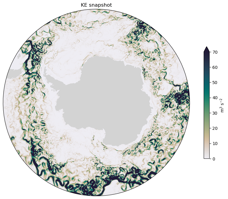
Snapshot plot of depth-integrated KE for a random time step:
[14]:
KE_snapshot = KE_dz.isel(time = 0).sum('st_ocean')
KE_snapshot = KE_snapshot.load()
[15]:
fig, axs = circumpolar_map()
KE_snapshot.plot(ax = axs, vmax = 70, cmap = cm.cm.rain, transform = ccrs.PlateCarree(),
                 cbar_kwargs = {'label':'m$^3$ s$^{-2}$', 'shrink':0.6});
axs.set_title('KE snapshot');
Mean Kinetic Energy
For the mean kinetic energy, we need to average the velocities over time.
[16]:
u_mean = u.mean('time')
v_mean = v.mean('time')
[17]:
MKE = (0.5*(u_mean**2 + v_mean**2)*dzu).sum('st_ocean')
[18]:
MKE = MKE.load()
[19]:
fig, axs = circumpolar_map()
MKE.plot(ax = axs, vmax = 70, cmap = cm.cm.rain, transform = ccrs.PlateCarree(),
         cbar_kwargs = {'label':'m$^3$ s$^{-2}$', 'shrink':0.6});
axs.set_title('MKE');
Eddy Kinetic Energy
We calculate the transient component of the velocity field and then compute the EKE:
[20]:
u_transient = u - u_mean
v_transient = v - v_mean
[21]:
EKE = (0.5*(u_transient**2 + v_transient**2)*dzu).sum('st_ocean').mean('time')
[22]:
EKE = EKE.load()
[23]:
fig, axs = circumpolar_map()
EKE.plot(ax = axs, vmax = 70, cmap = cm.cm.rain, transform = ccrs.PlateCarree(),
         cbar_kwargs = {'label':'m$^3$ s$^{-2}$', 'shrink':0.6});
axs.set_title('EKE');
[24]:
client.close()