Zonally Averaged Overturning Circulation
This notebook shows a simple example of calculation the zonally averaged global meridional overturning circulation - in density space - using output from either MOM5 or MOM6.
Requirements: The conda/analysis3 (or later) module on ARE. We recommend an ARE session with more than 14 cores to make these computations.
Firstly, load in the requisite libraries:
[1]:
%config InlineBackend.figure_format='retina'

import cosima_cookbook as cc
import matplotlib.pyplot as plt
import cmocean as cm
import numpy as np
from dask.distributed import Client
from scipy.interpolate import interp1d

import xarray as xr
import cf_xarray as cfxr
[2]:
client = Client(n_workers=14)
client
[2]:
Client
Client-25feb41c-7355-11ee-b605-000007b1fe80
| Connection method: Cluster object | Cluster type: distributed.LocalCluster |
| Dashboard: /proxy/45511/status |
Cluster Info
LocalCluster
c7091f40
| Dashboard: /proxy/45511/status | Workers: 14 |
| Total threads: 28 | Total memory: 112.00 GiB |
| Status: running | Using processes: True |
Scheduler Info
Scheduler
Scheduler-6a7f1f5e-17f8-492e-8c0d-3bd74d363033
| Comm: tcp://127.0.0.1:46879 | Workers: 14 |
| Dashboard: /proxy/45511/status | Total threads: 28 |
| Started: Just now | Total memory: 112.00 GiB |
Workers
Worker: 0
| Comm: tcp://127.0.0.1:41505 | Total threads: 2 |
| Dashboard: /proxy/40419/status | Memory: 8.00 GiB |
| Nanny: tcp://127.0.0.1:40795 | |
| Local directory: /jobfs/98961928.gadi-pbs/dask-scratch-space/worker-uqkij3lx | |
Worker: 1
| Comm: tcp://127.0.0.1:36939 | Total threads: 2 |
| Dashboard: /proxy/36815/status | Memory: 8.00 GiB |
| Nanny: tcp://127.0.0.1:39791 | |
| Local directory: /jobfs/98961928.gadi-pbs/dask-scratch-space/worker-u1iev5qr | |
Worker: 2
| Comm: tcp://127.0.0.1:40023 | Total threads: 2 |
| Dashboard: /proxy/42321/status | Memory: 8.00 GiB |
| Nanny: tcp://127.0.0.1:40853 | |
| Local directory: /jobfs/98961928.gadi-pbs/dask-scratch-space/worker-a5fucugz | |
Worker: 3
| Comm: tcp://127.0.0.1:34481 | Total threads: 2 |
| Dashboard: /proxy/36201/status | Memory: 8.00 GiB |
| Nanny: tcp://127.0.0.1:33451 | |
| Local directory: /jobfs/98961928.gadi-pbs/dask-scratch-space/worker-2p1gdw2q | |
Worker: 4
| Comm: tcp://127.0.0.1:33511 | Total threads: 2 |
| Dashboard: /proxy/42463/status | Memory: 8.00 GiB |
| Nanny: tcp://127.0.0.1:35551 | |
| Local directory: /jobfs/98961928.gadi-pbs/dask-scratch-space/worker-3c0wz7ly | |
Worker: 5
| Comm: tcp://127.0.0.1:44307 | Total threads: 2 |
| Dashboard: /proxy/41075/status | Memory: 8.00 GiB |
| Nanny: tcp://127.0.0.1:35705 | |
| Local directory: /jobfs/98961928.gadi-pbs/dask-scratch-space/worker-c4xdly_l | |
Worker: 6
| Comm: tcp://127.0.0.1:42855 | Total threads: 2 |
| Dashboard: /proxy/42225/status | Memory: 8.00 GiB |
| Nanny: tcp://127.0.0.1:46751 | |
| Local directory: /jobfs/98961928.gadi-pbs/dask-scratch-space/worker-nooiitdd | |
Worker: 7
| Comm: tcp://127.0.0.1:40121 | Total threads: 2 |
| Dashboard: /proxy/36093/status | Memory: 8.00 GiB |
| Nanny: tcp://127.0.0.1:38613 | |
| Local directory: /jobfs/98961928.gadi-pbs/dask-scratch-space/worker-regr2ejy | |
Worker: 8
| Comm: tcp://127.0.0.1:40075 | Total threads: 2 |
| Dashboard: /proxy/34999/status | Memory: 8.00 GiB |
| Nanny: tcp://127.0.0.1:33321 | |
| Local directory: /jobfs/98961928.gadi-pbs/dask-scratch-space/worker-vftq7992 | |
Worker: 9
| Comm: tcp://127.0.0.1:41165 | Total threads: 2 |
| Dashboard: /proxy/42749/status | Memory: 8.00 GiB |
| Nanny: tcp://127.0.0.1:41175 | |
| Local directory: /jobfs/98961928.gadi-pbs/dask-scratch-space/worker-zkenghtq | |
Worker: 10
| Comm: tcp://127.0.0.1:38401 | Total threads: 2 |
| Dashboard: /proxy/39299/status | Memory: 8.00 GiB |
| Nanny: tcp://127.0.0.1:42253 | |
| Local directory: /jobfs/98961928.gadi-pbs/dask-scratch-space/worker-15eamz_8 | |
Worker: 11
| Comm: tcp://127.0.0.1:43825 | Total threads: 2 |
| Dashboard: /proxy/46227/status | Memory: 8.00 GiB |
| Nanny: tcp://127.0.0.1:36393 | |
| Local directory: /jobfs/98961928.gadi-pbs/dask-scratch-space/worker-cw24zou7 | |
Worker: 12
| Comm: tcp://127.0.0.1:35653 | Total threads: 2 |
| Dashboard: /proxy/44945/status | Memory: 8.00 GiB |
| Nanny: tcp://127.0.0.1:45365 | |
| Local directory: /jobfs/98961928.gadi-pbs/dask-scratch-space/worker-0aodfyk_ | |
Worker: 13
| Comm: tcp://127.0.0.1:39967 | Total threads: 2 |
| Dashboard: /proxy/42007/status | Memory: 8.00 GiB |
| Nanny: tcp://127.0.0.1:34721 | |
| Local directory: /jobfs/98961928.gadi-pbs/dask-scratch-space/worker-givrgpu9 | |
At this stage, you need to denote whether the experiment uses output from MOM5 or MOM6.
This notebook is designed to use cf-xarray and a dictionary of querying.getvar arguments to load the correct variables independent of the model.
[3]:
session = cc.database.create_session()
Next, choose an experiment. The dictionary below denotes which experiment we want to use for each model.
We can choose experiments at any resolution. For MOM5-based runs, they can be with or without Gent-McWilliams eddy parameterisation.
For this example, we are choosing to limit ourselves to just the last 20 years of the 0.25° control simulations. If you want to increase the resolution or integrate over a longer time you might need more resources!
[4]:
psi_args = {
    "mom5": {
        "expt": "01deg_jra55v13_ryf9091",
        "variable": "ty_trans_rho",
        "start_time": "2152-01-01",
        "end_time": "2154-12-31",
        "chunks": {"time": 1,"potrho": -1,"grid_yu_ocean": 270,"grid_xt_ocean": -1,}
    },
    "mom6": {
        "expt": "global-01-v3",
        "variable": "vmo",
        "start_time": "2001-01-01",
        "end_time": "2002-01-01",
        "frequency": "1 monthly",
        "attrs": {"cell_methods": "rho2_l:sum yq:point xh:sum time: mean"},
    }
}
setting the dictionary for the remapping function:
[5]:
remap_dens = {
    "mom5": {
        "expt": "01deg_jra55v13_ryf9091",
        "frequency": "1 monthly",
        "rho_2" : "pot_rho_2",
        "depth" : "st_ocean",
        "latitude_c": "yt_ocean",
        "latitude_b": "yu_ocean",
        "latitude_bsect": "grid_yu_ocean",
        "chunks": {"time": 1, "potrho": -1, "grid_yu_ocean": 270, "grid_xt_ocean": -1}
    },
    "mom6": {
        "expt": "global-01-v3",
        "frequency": "1 monthly",
        "rho_2" : "rhopot2",
        "depth" : "z_l",
        "latitude_c": "yh",
        "latitude_b": "yq",
        "latitude_bsect": "yq",
        "attrs": {"cell_methods": "rho2_l:sum yq:point xh:sum time: mean"},
    }
}
Defining the remapping function
[6]:
def remap_depth(remap_dens,psi_args,psi_avg,session,model):
    rho2 = cc.querying.getvar(psi_args[model]["expt"], remap_dens[model]["rho_2"], session, start_time=psi_args[model]["start_time"], end_time=psi_args[model]["end_time"]).astype('float64')

    #Mask the Mediteranean
    if model=='mom5': rho2=rho2.where(((rho2.xt_ocean<0) | (rho2.xt_ocean>45) ) | ((rho2.yt_ocean<10) | (rho2.yt_ocean>48)))
    if model=='mom6': rho2=rho2.where(((rho2.xh<0) | (rho2.xh>45) ) | ((rho2.yh<10) | (rho2.yh>48)))

    rho2_mean = rho2.sel(time=slice(psi_args[model]["start_time"], psi_args[model]["end_time"])).mean('time')
    rho2_zonal_mean = rho2_mean.cf.mean("longitude").load()

    if model=='mom5':
        nmax=np.size(rho2_zonal_mean.yt_ocean)
        nmin=59
    elif model=='mom6':
        nmax=np.size(rho2_zonal_mean.yh)
        nmin=int(list(rho2_zonal_mean.yh.values).index(rho2_zonal_mean.sel(yh=-78, method='nearest').yh)) #locates lat=-78

    z1 = rho2_zonal_mean[remap_dens[model]["depth"]].values
    psi_depth = psi_avg.copy()*0.0
    for ii in range(nmin,nmax):
        if model=='mom5':
            rho1 = rho2_zonal_mean.isel(yt_ocean=ii); rho1v=rho1; z=rho1.st_ocean
            rho1 = rho1.rename({'st_ocean' : 'rho_ref'}); rho1['rho_ref']=np.array(rho1v)
            rho1.name='st_ocean'; rho1.values=np.array(z)
            rho1 = rho1.isel(rho_ref = ~np.isnan(rho1.rho_ref)).drop_duplicates(dim='rho_ref', keep='first')
            rho1 = rho1.interp(rho_ref = psi_avg.potrho.values, kwargs={"bounds_error": False, "fill_value": (0, 6000)})
            psi_depth[:, ii] = rho1.rename({'rho_ref' : 'potrho'})
        elif model=='mom6':
            rho1 = rho2_zonal_mean.isel(yh=ii); rho1v=rho1; z=rho1.z_l
            rho1 = rho1.rename({'z_l': 'rho_ref'}); rho1['rho_ref']=np.array(rho1v)
            rho1.name='z_l'; rho1.values=np.array(z)
            rho1 = rho1.isel(rho_ref = ~np.isnan(rho1.rho_ref)).drop_duplicates(dim='rho_ref', keep='first')
            rho1 = rho1.interp(rho_ref = psi_avg.rho2_l.values, kwargs={"bounds_error": False, "fill_value": (0, 6000)})
            psi_depth[:, ii] = rho1.rename({'rho_ref': 'rho2_l'})

    psi_avg2 = psi_avg.rename({remap_dens[model]["latitude_bsect"]: 'latitude_b'}) #Purely for automatic renaming later

    new_psi_avg = xr.DataArray(data = psi_avg2.values,
                               dims = [remap_dens[model]["rho_2"], 'latitude_b'],
                               coords = dict(latitude_b=(["latitude_b"], psi_avg2["latitude_b"].values),
                                           depth=([remap_dens[model]["rho_2"], "latitude_b"], psi_depth.values)),
                               attrs = psi_avg.attrs)

    new_psi_avg=new_psi_avg.rename({'latitude_b': remap_dens[model]["latitude_b"]})
    del psi_avg2

    return psi_depth, new_psi_avg
MOM5: Load up ty_trans_rho - and sum zonally. Also, if there is a ty_trans_rho_gm variable saved, assume that GM is switched on and load that as well. Most ACCESS-OM2 and MOM6 simulations save transport with units of kg/s - convert to Sv.
[7]:
def load_streamfunction(model):
    expt = psi_args[model]["expt"]
    start_time = psi_args[model]["start_time"]
    end_time = psi_args[model]["end_time"]

    psi = cc.querying.getvar(session=session, **psi_args[model])
    psi = psi.sel(time=slice(start_time, end_time))
    psi = psi.cf.sum("longitude")

    psiGM = xr.zeros_like(psi)

    varlist = cc.querying.get_variables(session, expt)
    if varlist['name'].str.contains('ty_trans_rho_gm').any():
        GM = True
        psiGM = cc.querying.getvar(expt, 'ty_trans_rho_gm', session, start_time=start_time)
        psiGM = psiGM.cf.sum("longitude")
    else:
        GM = False

    ρ0 = 1025 # mean density of sea-water [kg/m³]

    # convert to Sv
    psi = psi / (1e6 * ρ0)
    psiGM = psiGM / (1e6 * ρ0)

    return psi, psiGM, GM
Now, we define a function that cumulatively sums the transport in the vertical. Note that in MOM5 the ty_trans_rho_GM variable is computed differently and does not require summing in the vertical. Once the calculation has been laid out, we then load the variable to force the computation to occur.
[8]:
def sum_in_vertical(psi, psiGM, GM):
    psi_avg = psi.cf.cumsum("vertical").mean("time") - psi.cf.sum("vertical").mean("time")

    if GM:
        psi_avg = psi_avg + psiGM.cf.mean("time")

    psi_avg.load()

    return psi_avg
Let’s load everything from a MOM5 model.
[9]:
model = 'mom5'
psi, psiGM, GM = load_streamfunction(model)
psi_avg = sum_in_vertical(psi, psiGM, GM)
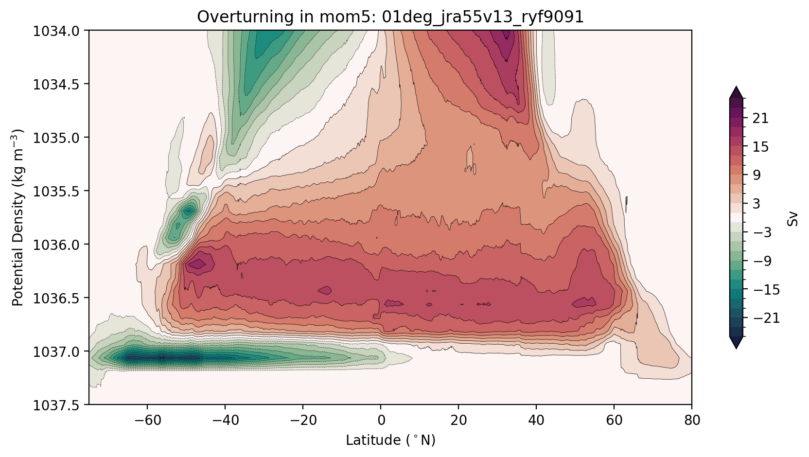
Now we are ready to plot. We usually plot the streamfunction over a reduced range of density levels to highlight the deep ocean contribution…
[10]:
plt.figure(figsize=(10, 5))

max_psi = 25 # Sv

# how we compute the levels may seem complicated, we just want to avoid a 0 contour
# so that the plot looks soothing to the eye
levels =  np.hstack((np.arange(-max_psi, 0, 2), np.flip(-np.arange(-max_psi, 0, 2))))
cbarticks = np.hstack((np.flip(-np.arange(3, max_psi, 6)), np.arange(3, max_psi, 6)))

psi_avg.plot.contourf(levels=levels,
                      cmap=cm.cm.curl, extend='both',
                      cbar_kwargs={'shrink': 0.7, 'label': 'Sv', 'ticks': cbarticks})

psi_avg.plot.contour(levels=levels, colors='k', linewidths=0.25)

plt.gca().invert_yaxis()

plt.ylim((1037.5, 1034))
plt.ylabel('Potential Density (kg m$^{-3}$)')
plt.xlabel('Latitude ($^\circ$N)')
plt.xlim([-75, 80])
plt.title(f'Overturning in {model}: {psi_args[model]["expt"]}');
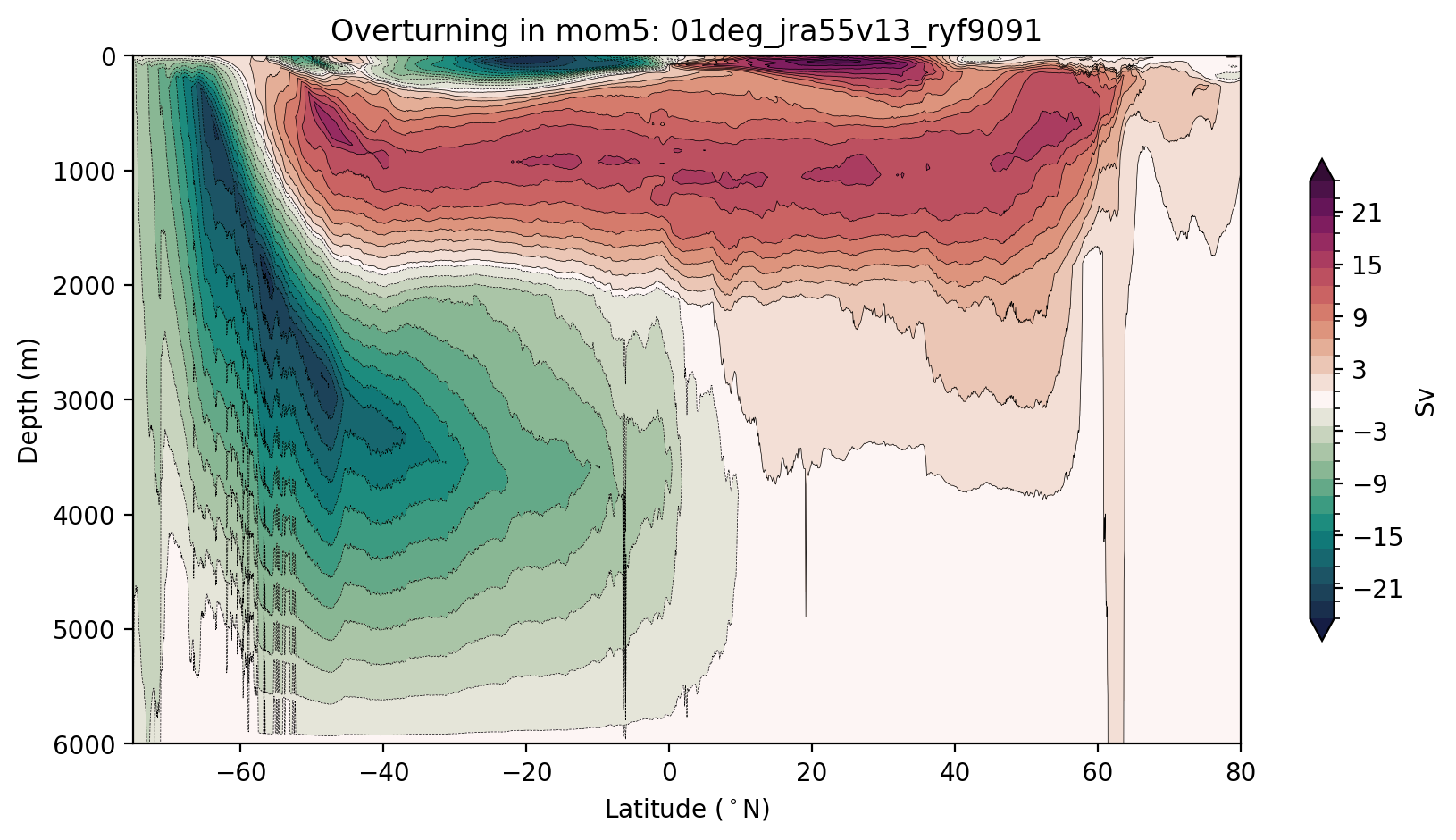
Now let’s remap the overturning into depth coordinates
[11]:
psi_depth, new_psi_avg = remap_depth(remap_dens, psi_args, psi_avg, session, model)
Plot of Streamfunction along depth
[12]:
plt.figure(figsize=(10, 5))

max_psi = 24.5 # Sv

# how we compute the levels may seem complicated, we just want to avoid a 0 contour
# so that the plot looks soothing to the eye
levels =  np.hstack((np.arange(-max_psi, 0, 2), np.flip(-np.arange(-max_psi, 0, 2))))
cbarticks = np.hstack((np.flip(-np.arange(3, max_psi, 6)), np.arange(3, max_psi, 6)))

new_psi_avg.plot.contourf(y="depth",levels=levels,
                      cmap=cm.cm.curl, extend='both',
                      cbar_kwargs={'shrink': 0.7, 'label': 'Sv', 'ticks': cbarticks})
new_psi_avg.plot.contour(y="depth",levels=levels, colors='k', linewidths=0.25)

plt.gca().invert_yaxis()


plt.ylabel('Depth (m)')
plt.xlabel('Latitude ($^\circ$N)')
plt.xlim([-75, 80])
plt.title(f'Overturning in {model}: {psi_args[model]["expt"]}');
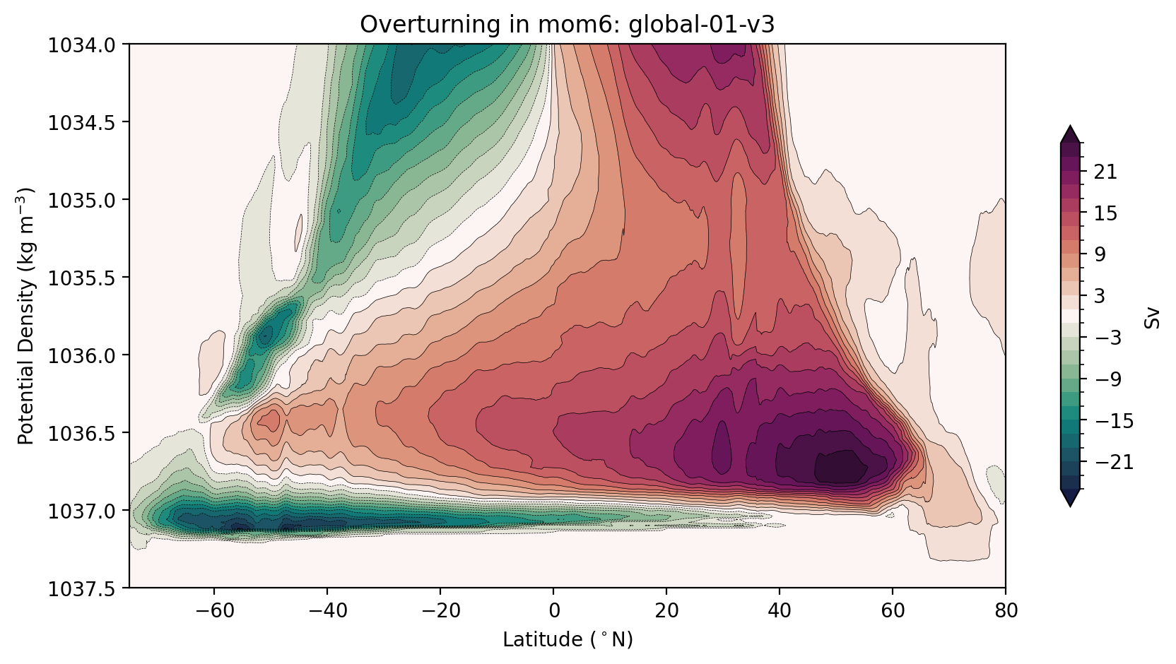
Now let’s do it again using output from a MOM6 model. Easy!
[13]:
model = 'mom6'
psi, psiGM, GM = load_streamfunction(model)
psi_avg = sum_in_vertical(psi, psiGM, GM)
[14]:
plt.figure(figsize=(10, 5))

max_psi = 25 # Sv

# how we compute the levels may seem complicated, we just want to avoid a 0 contour
# so that the plot looks soothing to the eye
levels =  np.hstack((np.arange(-max_psi, 0, 2), np.flip(-np.arange(-max_psi, 0, 2))))
cbarticks = np.hstack((np.flip(-np.arange(3, max_psi, 6)), np.arange(3, max_psi, 6)))

psi_avg.plot.contourf(levels=levels,
                      cmap=cm.cm.curl, extend='both',
                      cbar_kwargs={'shrink': 0.7, 'label': 'Sv', 'ticks': cbarticks})

psi_avg.plot.contour(levels=levels, colors='k', linewidths=0.25)

plt.gca().invert_yaxis()

plt.ylim((1037.5, 1034))
plt.ylabel('Potential Density (kg m$^{-3}$)')
plt.xlabel('Latitude ($^\circ$N)')
plt.xlim([-75, 80])
plt.title(f'Overturning in {model}: {psi_args[model]["expt"]}');
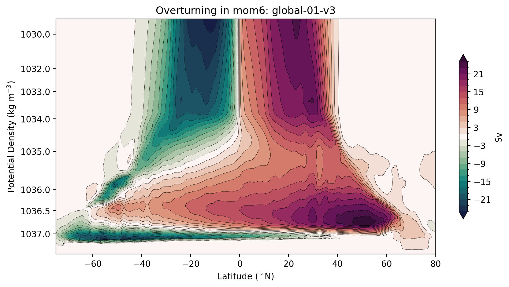
Alternatively, you may want to stretch your axes to minimise the visual impact of the surface circulation, while showing the full-depth ocean.
[15]:
stretching_factor = 4 # A powvalues set the stretching

ρmin = psi_avg.cf['vertical'].min()

psi_avg_plot = psi_avg.assign_coords(
    {
        psi_avg.cf["vertical"].name: (psi_avg.cf["vertical"] - ρmin)**stretching_factor
    }
)
[16]:
fig, ax = plt.subplots(1, 1, figsize=(10, 5))

max_psi = 25 # Sv

# how we compute the levels may seem complicated, we just want to avoid a 0 contour
# so that the plot looks soothing to the eye
levels =  np.hstack((np.arange(-max_psi, 0, 2), np.flip(-np.arange(-max_psi, 0, 2))))
cbarticks = np.hstack((np.flip(-np.arange(3, max_psi, 6)), np.arange(3, max_psi, 6)))

yticks = np.array([1030, 1032, 1033, 1034, 1035, 1036, 1036.5, 1037])

psi_avg_plot.plot.contourf(levels=levels,
                           cmap=cm.cm.curl, extend='both',
                           cbar_kwargs={'shrink': 0.7,'label': 'Sv', 'ticks': cbarticks})

psi_avg_plot.plot.contour(levels=levels, colors='k', linewidths=0.25)

plt.gca().set_yticks((yticks - ρmin.values)**stretching_factor)
plt.gca().set_yticklabels(yticks)

# ylims: a bit less than the minimnum and a bit more than the maximum values
plt.gca().set_ylim([((yticks - ρmin.values).min() / 1.1)**stretching_factor, ((yticks - ρmin.values).max() * 1.02)**stretching_factor])
plt.gca().invert_yaxis()

plt.ylabel('Potential Density (kg m$^{-3}$)')
plt.xlabel('Latitude ($^\circ$N)')
plt.xlim([-75, 80])
plt.title(f'Overturning in {model}: {psi_args[model]["expt"]}');
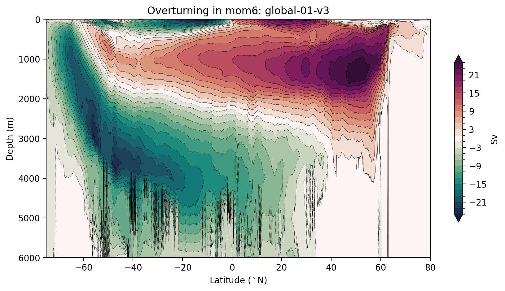
Remapping the mom6 streamfunction into depth coordinates.
[17]:
psi_depth, new_psi_avg = remap_depth(remap_dens, psi_args, psi_avg, session, model)
[ ]:
plt.figure(figsize=(10, 5))

max_psi = 25 # Sv

# how we compute the levels may seem complicated, we just want to avoid a 0 contour
# so that the plot looks soothing to the eye
levels =  np.hstack((np.arange(-max_psi, 0, 2), np.flip(-np.arange(-max_psi, 0, 2))))
cbarticks = np.hstack((np.flip(-np.arange(3, max_psi, 6)), np.arange(3, max_psi, 6)))

new_psi_avg.plot.contourf(y="depth",levels=levels,
                          cmap=cm.cm.curl, extend='both',
                          cbar_kwargs={'shrink': 0.7, 'label': 'Sv', 'ticks': cbarticks})
new_psi_avg.plot.contour(y="depth",levels=levels, colors='k', linewidths=0.25)

plt.gca().invert_yaxis()


plt.ylabel('Depth (m)')
plt.xlabel('Latitude ($^\circ$N)')
plt.xlim([-75, 80])
plt.title(f'Overturning in {model}: {psi_args[model]["expt"]}');
Notes:
We have not included the submesoscale contribution to the meridional transport in these calculations, as it tends to be relatively unimportant for the deep circulation, which we where we are primarily interested.
These metrics do not use mathematically correct zonal averaging in the tripole region, north of 65°N!