Relative Vorticity
This notebook shows a simple example of calculation the vertical component of relative vorticity,
For demonstration purposes we will compute the vorticity near the surface, but the method can be applied to any depth.
We will demonstrate three methods for computing relative voritcity:
A naïve method of simply converting degrees of longitude/latitude into metres and differentiating. This method works if you simply wanna have a look at how the vorticity field looks like.
A much more careful way of replicating exactly what the model does for computing the vertical component of relative vorticity.
A simpler but accurate method leveraging the functionality of the
xgcm.
Caveat: Both methods 2 and 3 automatically extend land masks into the domain, so needs extreme care if you care about coastlines! see https://github.com/xgcm/xgcm/issues/324
(To make a long story short: best method is probably method 3.)
Requirements: The conda/analysis3-20.01 (or later) module on the VDI/gadi (or your own up-to-date cookbook installation).
Firstly, load in the requisite libraries:
[1]:
%config InlineBackend.figure_format='retina'

import cosima_cookbook as cc
import matplotlib.pyplot as plt
import numpy as np
import cmocean as cm
from dask.distributed import Client

import matplotlib
from matplotlib import rc
rc('font',**{'family':'sans-serif'})
rc('text', usetex=False)

import xarray as xr
Load a dask client.
[2]:
client = Client()
client
[2]:
Client
Client-7cc78dc0-6054-11ee-badd-00000775fe80
| Connection method: Cluster object | Cluster type: distributed.LocalCluster |
| Dashboard: /proxy/8787/status |
Cluster Info
LocalCluster
a69178c7
| Dashboard: /proxy/8787/status | Workers: 7 |
| Total threads: 28 | Total memory: 112.00 GiB |
| Status: running | Using processes: True |
Scheduler Info
Scheduler
Scheduler-a8c7c6ff-5ca6-44a4-b053-30f0bf4493f4
| Comm: tcp://127.0.0.1:34265 | Workers: 7 |
| Dashboard: /proxy/8787/status | Total threads: 28 |
| Started: Just now | Total memory: 112.00 GiB |
Workers
Worker: 0
| Comm: tcp://127.0.0.1:37659 | Total threads: 4 |
| Dashboard: /proxy/42289/status | Memory: 16.00 GiB |
| Nanny: tcp://127.0.0.1:41035 | |
| Local directory: /jobfs/96729342.gadi-pbs/dask-scratch-space/worker-i9uh229j | |
Worker: 1
| Comm: tcp://127.0.0.1:43157 | Total threads: 4 |
| Dashboard: /proxy/43437/status | Memory: 16.00 GiB |
| Nanny: tcp://127.0.0.1:37761 | |
| Local directory: /jobfs/96729342.gadi-pbs/dask-scratch-space/worker-oyp28sq8 | |
Worker: 2
| Comm: tcp://127.0.0.1:38511 | Total threads: 4 |
| Dashboard: /proxy/36417/status | Memory: 16.00 GiB |
| Nanny: tcp://127.0.0.1:36385 | |
| Local directory: /jobfs/96729342.gadi-pbs/dask-scratch-space/worker-76u7daas | |
Worker: 3
| Comm: tcp://127.0.0.1:36487 | Total threads: 4 |
| Dashboard: /proxy/34003/status | Memory: 16.00 GiB |
| Nanny: tcp://127.0.0.1:41257 | |
| Local directory: /jobfs/96729342.gadi-pbs/dask-scratch-space/worker-kdq9gsjx | |
Worker: 4
| Comm: tcp://127.0.0.1:33941 | Total threads: 4 |
| Dashboard: /proxy/40241/status | Memory: 16.00 GiB |
| Nanny: tcp://127.0.0.1:40795 | |
| Local directory: /jobfs/96729342.gadi-pbs/dask-scratch-space/worker-g0nbndq7 | |
Worker: 5
| Comm: tcp://127.0.0.1:36181 | Total threads: 4 |
| Dashboard: /proxy/40343/status | Memory: 16.00 GiB |
| Nanny: tcp://127.0.0.1:33505 | |
| Local directory: /jobfs/96729342.gadi-pbs/dask-scratch-space/worker-c34tebb5 | |
Worker: 6
| Comm: tcp://127.0.0.1:33747 | Total threads: 4 |
| Dashboard: /proxy/39505/status | Memory: 16.00 GiB |
| Nanny: tcp://127.0.0.1:44827 | |
| Local directory: /jobfs/96729342.gadi-pbs/dask-scratch-space/worker-_qun4ltl | |
[3]:
expt = '025deg_jra55v13_iaf_gmredi6'
session = cc.database.create_session()
Various parameters that will be used for computing quantities.
[4]:
# these are the values used by MOM5

Ω = 7.292e-5     # Earth's rotation rate in radians/s
Rearth = 6371.e3 # Earth's radius in m
Load lon and lat used in the experiment. These datasets can be used for plotting.
[5]:
lon = cc.querying.getvar(expt, 'geolon_c', session, ncfile="ocean_grid.nc", n=1)
lat = cc.querying.getvar(expt, 'geolat_c', session, ncfile="ocean_grid.nc", n=1)
Calculate the Coriolis parameter \(f = 2\Omega \sin(\texttt{lat})\).
[6]:
f = 2 * Ω * np.sin(np.deg2rad(lat)) # convert lat in radians
f = f.rename('Coriolis')
f.attrs['long_name'] = 'Coriolis parameter'
f.attrs['units'] = 's-1'
f.attrs['coordinates'] = 'geolon_c geolat_c'
Load the \(u\) and \(v\) velocity snapshots. Then we pick a depth value below the Ekman layer, namely the closest to \(z=-30\,m\).
The code .isel(time=-1) selects the final snapshot of u or v. Remove .isel(time=-1) to load all available snapshots of the flow fields.
[7]:
depth = 30 #m; avoid the surface Ekman layer by taking the "surface values" at some depth close to the surface

u = cc.querying.getvar(expt, 'u', session, ncfile="ocean.nc")
u = u.isel(time=-1).sel(st_ocean=depth, method='nearest')

v = cc.querying.getvar(expt, 'v', session, ncfile="ocean.nc")
v = v.isel(time=-1).sel(st_ocean=depth, method='nearest')
Method 1 (naïve computation)
To compute relative vorticity \(\zeta = \partial_x v - \partial_y u\) we simply differentiate the velocity components with respect of lon (here xu_ocean in degrees) and lat (here yu_ocean in degrees). We then convert the derivatives from units of degrees\(^{-1}\) to m\(^{-1}\). To do so, we use the value of the radius of the Earth Rearth and also take into account that as we go towards the poles the lon-grid spacing is scaled by \(\cos(\) lat
\()\).
(Note the unicode characters like ζ can be used in python.)
[8]:
ζ_naive = v.differentiate('xu_ocean') / np.deg2rad(Rearth*np.cos(np.deg2rad(lat))) - u.differentiate('yu_ocean') / (np.pi/180*Rearth)
ζ_naive = ζ_naive.rename('Relative Vorticity')
ζ_naive.attrs['long_name'] = 'Relative Vorticity, ∂v/∂x-∂u/∂y'
ζ_naive.attrs['units'] = 's-1'
[9]:
ζ_naive
[9]:
<xarray.DataArray 'Relative Vorticity' (yu_ocean: 1080, xu_ocean: 1440)>
dask.array<sub, shape=(1080, 1440), dtype=float32, chunksize=(216, 288), chunktype=numpy.ndarray>
Coordinates:
    st_ocean  float64 30.36
    time      datetime64[ns] 2257-06-30T12:00:00
  * xu_ocean  (xu_ocean) float64 -279.8 -279.5 -279.2 -279.0 ... 79.5 79.75 80.0
  * yu_ocean  (yu_ocean) float64 -81.02 -80.92 -80.81 ... 89.79 89.89 90.0
    geolon_c  (yu_ocean, xu_ocean) float32 dask.array<chunksize=(540, 720), meta=np.ndarray>
    geolat_c  (yu_ocean, xu_ocean) float32 dask.array<chunksize=(540, 720), meta=np.ndarray>
Attributes:
    long_name:  Relative Vorticity, ∂v/∂x-∂u/∂y
units: s-1We now plot \(\zeta\) in the North Atlantic.
[10]:
maxvalue = 6e-6
levels = np.linspace(-maxvalue, maxvalue, 24)
[11]:
fig = plt.figure(figsize=(10, 5))
ζ_naive.plot.contourf(levels=levels, x='geolon_c', y='geolat_c', cmap="RdBu_r", vmin=-maxvalue, vmax=maxvalue, extend='both', add_labels=False)
plt.title("snapshot of relative vorticity, $\zeta = \partial_x v - \partial_y u$ [naïve]");
plt.xlabel("longitude")
plt.ylabel("latitude")
plt.xlim(-120, 20)
plt.ylim(20, 90);
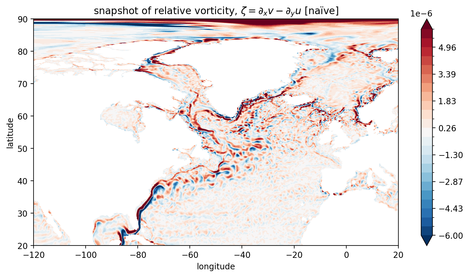
This method is sort-of-OK below 65N where the complications of the tripolar grid do not enter. But even south of 65N this method gives a rough estimate. It’s OK for visualising but it should not be used in computing, e.g., vorticity budgets.
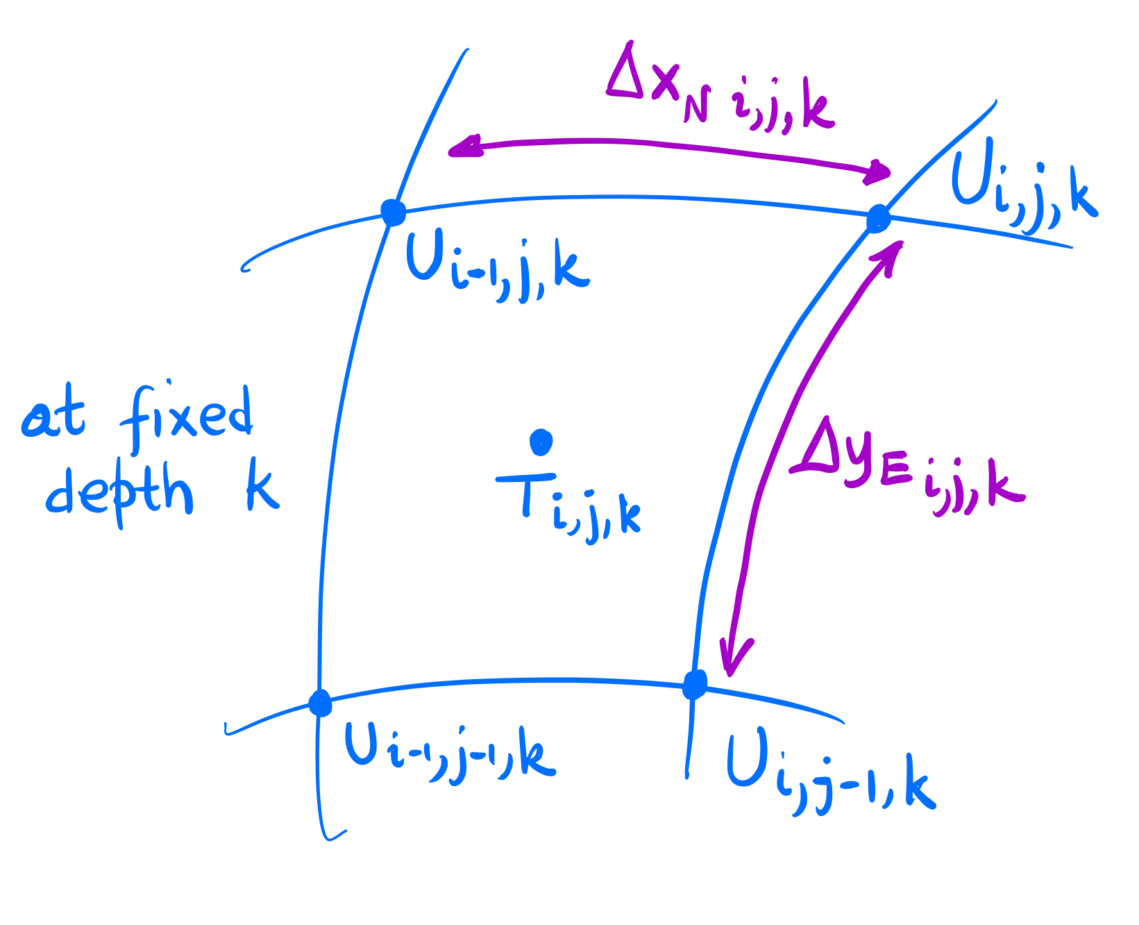
Method 2: replicating how MOM5 computes vorticity_z
Looking at MOM5 code and by doing some translation from Fortran code to “english” we can see that the models computes vorticity_z via:
Above, \((i, j, k)\) refers to the grid-point indices for directions \(x, y, z\) respectively.
The distances \(\Delta x_N\) and \(\Delta y_E\) correspond to the North and East faces of the corresponding \(T\)-cell; see the diagram below. (T-points are those in the cells’s centres where tracers are evaluated and U-points are in the cells’s corners where velocities are evaluated.)
[12]:
ds_grid = xr.open_mfdataset('/g/data/hh5/tmp/cosima/access-om2-025/025deg_jra55v13_iaf_gmredi6/output000/ocean/ocean_grid.nc', combine='by_coords')
ds = xr.merge([u, v, ds_grid])
After a lot of fiddling with indiced you can confirm that the right way to compute \(\delta x_N\) and \(\delta y_E\) from above is:
[13]:
inverse_dxtn = 0.5*(1/ds.dxu + np.roll(1/ds.dxu, 1, axis=1))
inverse_dyte = 0.5*(1/ds.dyu + np.roll(1/ds.dyu, 1, axis=0))
… and with that we can now compute ζ_mom5 which is the vorticity as exactly the way is computed by the model:
[14]:
vx_ijk = (ds.v - np.roll(ds.v, 1, axis=1))*inverse_dxtn
uy_ijk = (ds.u - np.roll(ds.u, 1, axis=0))*inverse_dyte

vx = 0.5 * (vx_ijk + np.roll(vx_ijk, 1, axis=0))
uy = 0.5 * (uy_ijk + np.roll(uy_ijk, 1, axis=1))

ζ_mom5 = vx - uy
The way we computed ζ_mom5 above using numpy.roll is not really ideal. One would like to do the above using xarray’s functionality… But, as we will argue below, you shouldn’t be using this way anyway because it’s cumbersome and it requires you to know the specifics of the staggered grid used in the model (Arakawa B-grid for MOM5). A way to avoid getting into the nitty-gritty of staggered grids is to use xgcm packaged (described in Method 3).
With this and that let’s plot ζ_mom5.
[15]:
fig = plt.figure(figsize=(10, 5))
ζ_mom5.plot.contourf(levels=levels, x='geolon_c', y='geolat_c', cmap="RdBu_r", vmin=-maxvalue, vmax=maxvalue, extend='both', add_labels=False)
plt.title("snapshot of relative vorticity, $\zeta = \partial_x v - \partial_y u$ [as in MOM5]")
plt.xlabel("longitude")
plt.ylabel("latitude")
plt.xlim(-120, 20)
plt.ylim(20, 90);
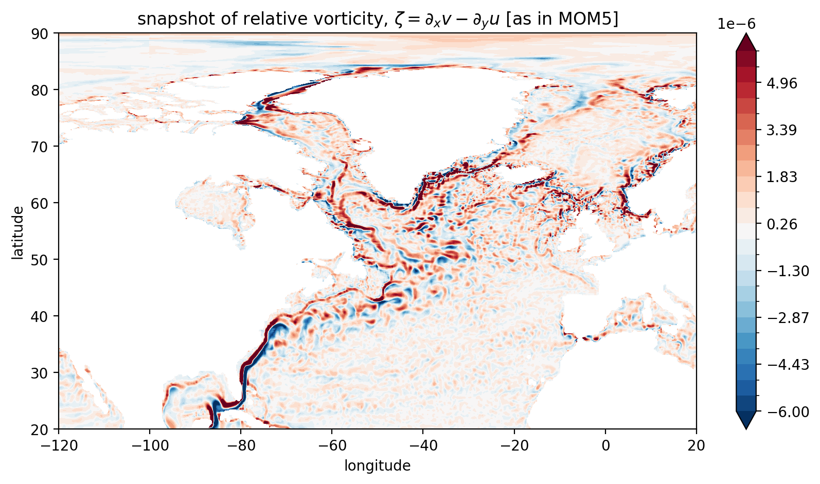
Note that the Arctic region now looks more “reasonable”.
Method 3: Using xgcm to replicate MOM5’s calculation for vorticity_z
`xgcm <https://xgcm.readthedocs.io/en/stable/>`__ is a package that deals with staggered grids that are typically used in ocean models. An excerpt from xgcm’s docs mentions:
“(in model output datasets), different variables are located at different positions with respect to a volume or area element (e.g. cell center, cell face, etc.) xgcm solves the problem of how to interpolate and difference these variables from one position to another.”
[16]:
import xgcm
print("xgcm version ", xgcm.__version__)
xgcm version 0.8.1
The way xgcm works is that we first create a grid object that has all the information regarding our staggered grid. For our case, grid needs to know the location of the xt_ocean, xu_ocean points (and same for \(y\)) and their relative orientation to one another, i.e., that xu_ocean is shifted to the right of xt_ocean by \(\frac1{2}\) grid-cell.
[17]:
folder = '/g/data/hh5/tmp/cosima/access-om2-025/025deg_jra55v13_iaf_gmredi6/output000/ocean/'
grid = xr.open_mfdataset(folder+'ocean_grid.nc', combine='by_coords')

ds = xr.merge([u, v, grid])
ds.coords['xt_ocean'].attrs.update(axis='X')
ds.coords['xu_ocean'].attrs.update(axis='X', c_grid_axis_shift=0.5)
ds.coords['yt_ocean'].attrs.update(axis='Y')
ds.coords['yu_ocean'].attrs.update(axis='Y', c_grid_axis_shift=0.5)

grid = xgcm.Grid(ds, periodic=['X'])
Then, xgcm give you a way to interpolate between grids (with the .interp function) and a way to compute differences (.diff function). For example, the exrpession \(v(i,j,k) - v(i-1,j,k)\) is obtained via grid.diff(ds.v, 'X').
Using xgcm’s functionality we can replicate the MOM5 vertical vorticity computation as:
[18]:
ζ_xgcm = ( grid.interp( grid.diff(ds.v, 'X') / grid.interp(ds.dxu, 'X'), 'Y', boundary='extend')
          - grid.interp( grid.diff(ds.u, 'Y', boundary='extend') / grid.interp(ds.dyt, 'X'), 'X') )

ζ_xgcm = ζ_xgcm.rename('Relative Vorticity')
ζ_xgcm.attrs['long_name'] = 'Relative Vorticity, ∂v/∂x-∂u/∂y'
ζ_xgcm.attrs['units'] = 's-1'
(Note: A simpler expression for ζ_xgcm could be:
ζ_xgcm = grid.interp(grid.diff(ds.v, 'X'), 'Y', boundary='extend')/ds.dxt - grid.interp(grid.diff(ds.u, 'Y', boundary='extend'), 'X')/ds.dyt
However, the above does not replicate precisely the way MOM5 computes vorticity_z.)
Now, let’s plot ζ_xgcm…
[19]:
fig = plt.figure(figsize=(10, 5))
ax = fig.add_subplot(1, 1, 1)
p = ax.contourf(lon, lat, ζ_xgcm.values, levels=levels, cmap="RdBu_r", vmin=-maxvalue, vmax=maxvalue, extend='both')
ax.set_title("snapshot of relative vorticity, $\zeta = \partial_x v - \partial_y u$ [by xgcm]")
plt.colorbar(p, extend='both')
plt.xlim(-120, 20)
plt.ylim(20, 90);
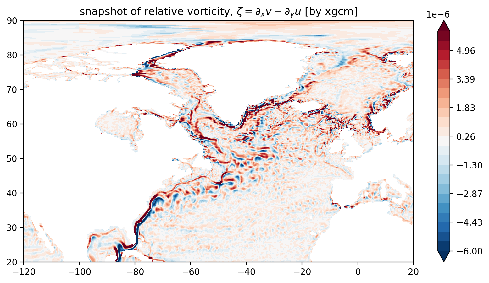
Looks OK and it was definitely easier than method 2.
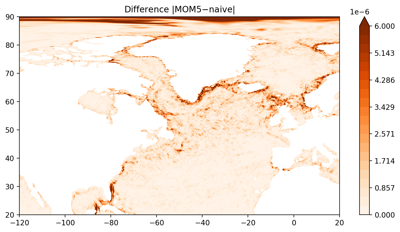
Comparison of the three methods
Now let’s be thorough and compare the vorticities computed via the three methods.
[20]:
fig = plt.figure(figsize=(10, 5))
ax = fig.add_subplot(1, 1, 1)
p = ax.contourf(lon, lat, np.abs(ζ_mom5.values-ζ_naive.values), levels=np.linspace(0, maxvalue, 22), cmap="Oranges", vmin=0, vmax=maxvalue, extend='max')
ax.set_title("Difference $|$MOM5$-$naive$|$")
plt.colorbar(p, extend='both')
plt.xlim(-120, 20)
plt.ylim(20, 90);
[21]:
fig = plt.figure(figsize=(10, 5))
ax = fig.add_subplot(1, 1, 1)
p = ax.contourf(lon, lat, np.abs(ζ_mom5.values-ζ_xgcm.values), levels=np.linspace(0, maxvalue, 22), cmap="Oranges", vmin=0, vmax=maxvalue, extend='max')
ax.set_title("Difference $|$MOM5$-$xgcm$|$");
plt.colorbar(p, extend='max')
plt.xlim(-120, 20)
plt.ylim(20, 90);
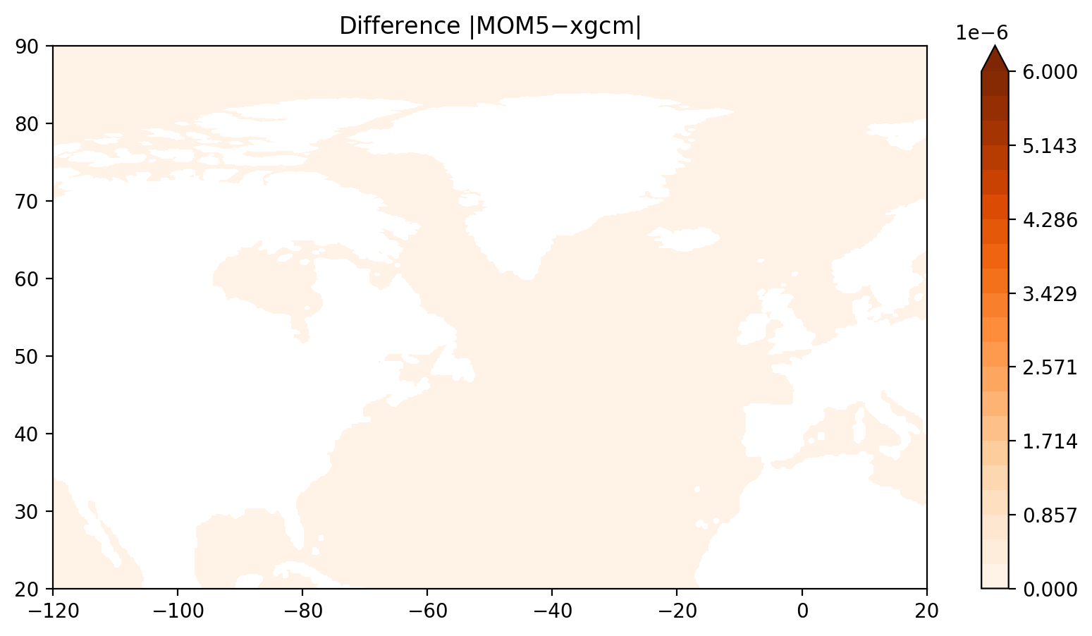
Indeed the xgcm method gives the same as the MOM5 code.
We have confirmed that indeed ζ_mom5 corresponds exactly to the vorticity_z diagnostic that the model outputs. To test this, the model was run for 1 day, save u, v and vorticity_z and then confirm that the ζ_mom5 computation from method 2 is equal to vorticity_z (up to machine precision). For brevity this comparison is not included here.
Further Potential Improvements on Method 3
xgcm has a functionality to perform derivatives and interpolations using the grid metrics. Implementing that would simplify the vorticity calculations even more, e.g.,
ζ_xgcm = grid.derivative(ds.v, 'X') - grid.derivative(ds.u, 'Y')
Something like that would be terrific; the user will only have to type up the algebraic expression of what they want to compute without any reference to dxt or dxu distances…
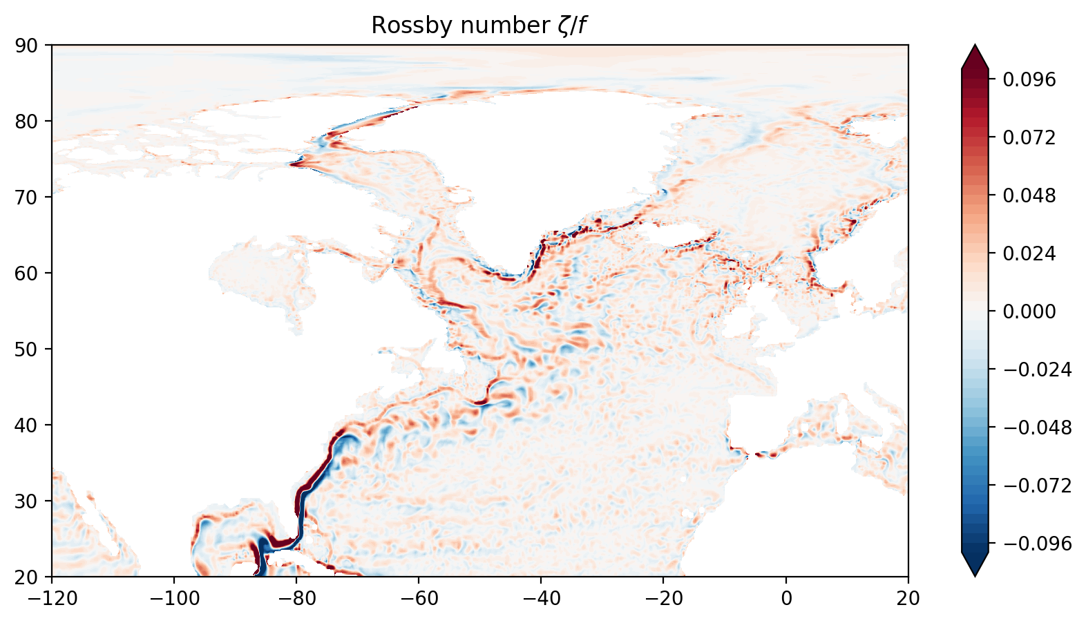
The Rossby number
To conclude, let’s visualize the Rossby number
where \(f=2\Omega\sin(\theta)\) is the Coriolis parameter.
[22]:
f = grid.interp(grid.interp(f, 'X'), 'Y', boundary='extend')
[23]:
Ro = ζ_xgcm/f
Ro = Ro.rename('Rossby number ζ/f')

fig = plt.figure(figsize=(10, 5))
ax = fig.add_subplot(1, 1, 1)
p = ax.contourf(lon, lat, Ro, levels=np.linspace(-0.1, 0.1, 51), cmap="RdBu_r", vmin=-0.1, vmax=0.1, extend='both')
ax.set_title("Rossby number $\zeta/f$")
plt.colorbar(p, extend='both')
plt.xlim(-120, 20)
plt.ylim(20, 90);