Regional Tasmanian domain forced by JRA55-do reanalysis and ACCESS-OM2-01 model output
What does this recipe do?
This recipe uses regional-mom6 package to set up a regional ocean configuration with MOM6. The recipe uses input from:
Input Type |
Source |
Location on NCI |
|---|---|---|
Surface |
|
|
Ocean |
|
|
Bathymetry |
|
Additionally to access to project ik11, we also need access to /g/data/x77 if we want to use the same executable using the latest FMS build (which is a good idea for troubleshooting).
[1]:
import intake
import xarray as xr
import os
import subprocess
import matplotlib.pyplot as plt
from pathlib import Path
from dask.distributed import Client

import regional_mom6 as rmom6
print("using regional-mom6 version " + rmom6.__version__)
using regional-mom6 version 1.0.1
Start a dask client.
[2]:
client = Client(threads_per_worker = 1)
client
[2]:
Client
Client-9ea0baca-ba06-11f0-a18a-0000008dfe80
| Connection method: Cluster object | Cluster type: distributed.LocalCluster |
| Dashboard: /proxy/8787/status |
Cluster Info
LocalCluster
93acb5d6
| Dashboard: /proxy/8787/status | Workers: 48 |
| Total threads: 48 | Total memory: 188.56 GiB |
| Status: running | Using processes: True |
Scheduler Info
Scheduler
Scheduler-9359a6df-1367-4852-b5d8-41ed82f2230d
| Comm: tcp://127.0.0.1:40149 | Workers: 0 |
| Dashboard: /proxy/8787/status | Total threads: 0 |
| Started: Just now | Total memory: 0 B |
Workers
Worker: 0
| Comm: tcp://127.0.0.1:44893 | Total threads: 1 |
| Dashboard: /proxy/35015/status | Memory: 3.93 GiB |
| Nanny: tcp://127.0.0.1:42067 | |
| Local directory: /jobfs/154022484.gadi-pbs/dask-scratch-space/worker-hoo5w9cs | |
Worker: 1
| Comm: tcp://127.0.0.1:45733 | Total threads: 1 |
| Dashboard: /proxy/36129/status | Memory: 3.93 GiB |
| Nanny: tcp://127.0.0.1:39189 | |
| Local directory: /jobfs/154022484.gadi-pbs/dask-scratch-space/worker-i8dikepm | |
Worker: 2
| Comm: tcp://127.0.0.1:35661 | Total threads: 1 |
| Dashboard: /proxy/39949/status | Memory: 3.93 GiB |
| Nanny: tcp://127.0.0.1:41049 | |
| Local directory: /jobfs/154022484.gadi-pbs/dask-scratch-space/worker-a3twoc2w | |
Worker: 3
| Comm: tcp://127.0.0.1:39683 | Total threads: 1 |
| Dashboard: /proxy/33083/status | Memory: 3.93 GiB |
| Nanny: tcp://127.0.0.1:36123 | |
| Local directory: /jobfs/154022484.gadi-pbs/dask-scratch-space/worker-ewn7o5jz | |
Worker: 4
| Comm: tcp://127.0.0.1:43069 | Total threads: 1 |
| Dashboard: /proxy/37715/status | Memory: 3.93 GiB |
| Nanny: tcp://127.0.0.1:46083 | |
| Local directory: /jobfs/154022484.gadi-pbs/dask-scratch-space/worker-_dmkogfi | |
Worker: 5
| Comm: tcp://127.0.0.1:43849 | Total threads: 1 |
| Dashboard: /proxy/37405/status | Memory: 3.93 GiB |
| Nanny: tcp://127.0.0.1:33919 | |
| Local directory: /jobfs/154022484.gadi-pbs/dask-scratch-space/worker-_53iohhi | |
Worker: 6
| Comm: tcp://127.0.0.1:36993 | Total threads: 1 |
| Dashboard: /proxy/45487/status | Memory: 3.93 GiB |
| Nanny: tcp://127.0.0.1:41633 | |
| Local directory: /jobfs/154022484.gadi-pbs/dask-scratch-space/worker-7hw9rmnf | |
Worker: 7
| Comm: tcp://127.0.0.1:34261 | Total threads: 1 |
| Dashboard: /proxy/41187/status | Memory: 3.93 GiB |
| Nanny: tcp://127.0.0.1:42271 | |
| Local directory: /jobfs/154022484.gadi-pbs/dask-scratch-space/worker-l6z241la | |
Worker: 8
| Comm: tcp://127.0.0.1:44577 | Total threads: 1 |
| Dashboard: /proxy/35955/status | Memory: 3.93 GiB |
| Nanny: tcp://127.0.0.1:41535 | |
| Local directory: /jobfs/154022484.gadi-pbs/dask-scratch-space/worker-z9b10cv7 | |
Worker: 9
| Comm: tcp://127.0.0.1:41653 | Total threads: 1 |
| Dashboard: /proxy/46757/status | Memory: 3.93 GiB |
| Nanny: tcp://127.0.0.1:42145 | |
| Local directory: /jobfs/154022484.gadi-pbs/dask-scratch-space/worker-3_bq1u6f | |
Worker: 10
| Comm: tcp://127.0.0.1:35501 | Total threads: 1 |
| Dashboard: /proxy/39223/status | Memory: 3.93 GiB |
| Nanny: tcp://127.0.0.1:43597 | |
| Local directory: /jobfs/154022484.gadi-pbs/dask-scratch-space/worker-gfc8cwqy | |
Worker: 11
| Comm: tcp://127.0.0.1:34415 | Total threads: 1 |
| Dashboard: /proxy/45981/status | Memory: 3.93 GiB |
| Nanny: tcp://127.0.0.1:38283 | |
| Local directory: /jobfs/154022484.gadi-pbs/dask-scratch-space/worker-083z1xgd | |
Worker: 12
| Comm: tcp://127.0.0.1:40921 | Total threads: 1 |
| Dashboard: /proxy/37471/status | Memory: 3.93 GiB |
| Nanny: tcp://127.0.0.1:40237 | |
| Local directory: /jobfs/154022484.gadi-pbs/dask-scratch-space/worker-l4zbh57f | |
Worker: 13
| Comm: tcp://127.0.0.1:40999 | Total threads: 1 |
| Dashboard: /proxy/37689/status | Memory: 3.93 GiB |
| Nanny: tcp://127.0.0.1:37511 | |
| Local directory: /jobfs/154022484.gadi-pbs/dask-scratch-space/worker-10l8wrto | |
Worker: 14
| Comm: tcp://127.0.0.1:35583 | Total threads: 1 |
| Dashboard: /proxy/36557/status | Memory: 3.93 GiB |
| Nanny: tcp://127.0.0.1:43829 | |
| Local directory: /jobfs/154022484.gadi-pbs/dask-scratch-space/worker-2hmypd6p | |
Worker: 15
| Comm: tcp://127.0.0.1:34149 | Total threads: 1 |
| Dashboard: /proxy/35891/status | Memory: 3.93 GiB |
| Nanny: tcp://127.0.0.1:33997 | |
| Local directory: /jobfs/154022484.gadi-pbs/dask-scratch-space/worker-nhdnpit6 | |
Worker: 16
| Comm: tcp://127.0.0.1:41257 | Total threads: 1 |
| Dashboard: /proxy/32929/status | Memory: 3.93 GiB |
| Nanny: tcp://127.0.0.1:36025 | |
| Local directory: /jobfs/154022484.gadi-pbs/dask-scratch-space/worker-lpohu85w | |
Worker: 17
| Comm: tcp://127.0.0.1:35159 | Total threads: 1 |
| Dashboard: /proxy/44685/status | Memory: 3.93 GiB |
| Nanny: tcp://127.0.0.1:34281 | |
| Local directory: /jobfs/154022484.gadi-pbs/dask-scratch-space/worker-9e74mhiv | |
Worker: 18
| Comm: tcp://127.0.0.1:43443 | Total threads: 1 |
| Dashboard: /proxy/46097/status | Memory: 3.93 GiB |
| Nanny: tcp://127.0.0.1:33719 | |
| Local directory: /jobfs/154022484.gadi-pbs/dask-scratch-space/worker-633x802b | |
Worker: 19
| Comm: tcp://127.0.0.1:34465 | Total threads: 1 |
| Dashboard: /proxy/45057/status | Memory: 3.93 GiB |
| Nanny: tcp://127.0.0.1:44681 | |
| Local directory: /jobfs/154022484.gadi-pbs/dask-scratch-space/worker-twq8tucx | |
Worker: 20
| Comm: tcp://127.0.0.1:37213 | Total threads: 1 |
| Dashboard: /proxy/41961/status | Memory: 3.93 GiB |
| Nanny: tcp://127.0.0.1:36829 | |
| Local directory: /jobfs/154022484.gadi-pbs/dask-scratch-space/worker-ee60m9nx | |
Worker: 21
| Comm: tcp://127.0.0.1:35647 | Total threads: 1 |
| Dashboard: /proxy/44257/status | Memory: 3.93 GiB |
| Nanny: tcp://127.0.0.1:33325 | |
| Local directory: /jobfs/154022484.gadi-pbs/dask-scratch-space/worker-ek45_v7k | |
Worker: 22
| Comm: tcp://127.0.0.1:38127 | Total threads: 1 |
| Dashboard: /proxy/37273/status | Memory: 3.93 GiB |
| Nanny: tcp://127.0.0.1:35255 | |
| Local directory: /jobfs/154022484.gadi-pbs/dask-scratch-space/worker-yrw57nj5 | |
Worker: 23
| Comm: tcp://127.0.0.1:46629 | Total threads: 1 |
| Dashboard: /proxy/42565/status | Memory: 3.93 GiB |
| Nanny: tcp://127.0.0.1:37713 | |
| Local directory: /jobfs/154022484.gadi-pbs/dask-scratch-space/worker-2g7eui6n | |
Worker: 24
| Comm: tcp://127.0.0.1:45525 | Total threads: 1 |
| Dashboard: /proxy/46543/status | Memory: 3.93 GiB |
| Nanny: tcp://127.0.0.1:33173 | |
| Local directory: /jobfs/154022484.gadi-pbs/dask-scratch-space/worker-nj8oso9d | |
Worker: 25
| Comm: tcp://127.0.0.1:36757 | Total threads: 1 |
| Dashboard: /proxy/46733/status | Memory: 3.93 GiB |
| Nanny: tcp://127.0.0.1:33341 | |
| Local directory: /jobfs/154022484.gadi-pbs/dask-scratch-space/worker-77nwy48k | |
Worker: 26
| Comm: tcp://127.0.0.1:34773 | Total threads: 1 |
| Dashboard: /proxy/40497/status | Memory: 3.93 GiB |
| Nanny: tcp://127.0.0.1:36579 | |
| Local directory: /jobfs/154022484.gadi-pbs/dask-scratch-space/worker-cbjvd_a1 | |
Worker: 27
| Comm: tcp://127.0.0.1:34889 | Total threads: 1 |
| Dashboard: /proxy/37321/status | Memory: 3.93 GiB |
| Nanny: tcp://127.0.0.1:34039 | |
| Local directory: /jobfs/154022484.gadi-pbs/dask-scratch-space/worker-i4fi3w9y | |
Worker: 28
| Comm: tcp://127.0.0.1:38303 | Total threads: 1 |
| Dashboard: /proxy/34381/status | Memory: 3.93 GiB |
| Nanny: tcp://127.0.0.1:45967 | |
| Local directory: /jobfs/154022484.gadi-pbs/dask-scratch-space/worker-lfmodjem | |
Worker: 29
| Comm: tcp://127.0.0.1:38939 | Total threads: 1 |
| Dashboard: /proxy/37413/status | Memory: 3.93 GiB |
| Nanny: tcp://127.0.0.1:39443 | |
| Local directory: /jobfs/154022484.gadi-pbs/dask-scratch-space/worker-gg14_au2 | |
Worker: 30
| Comm: tcp://127.0.0.1:36201 | Total threads: 1 |
| Dashboard: /proxy/35885/status | Memory: 3.93 GiB |
| Nanny: tcp://127.0.0.1:44597 | |
| Local directory: /jobfs/154022484.gadi-pbs/dask-scratch-space/worker-r_dxjw1j | |
Worker: 31
| Comm: tcp://127.0.0.1:34535 | Total threads: 1 |
| Dashboard: /proxy/37721/status | Memory: 3.93 GiB |
| Nanny: tcp://127.0.0.1:46113 | |
| Local directory: /jobfs/154022484.gadi-pbs/dask-scratch-space/worker-lvnf_vcl | |
Worker: 32
| Comm: tcp://127.0.0.1:46707 | Total threads: 1 |
| Dashboard: /proxy/43647/status | Memory: 3.93 GiB |
| Nanny: tcp://127.0.0.1:43891 | |
| Local directory: /jobfs/154022484.gadi-pbs/dask-scratch-space/worker-ecv19rqc | |
Worker: 33
| Comm: tcp://127.0.0.1:38059 | Total threads: 1 |
| Dashboard: /proxy/44353/status | Memory: 3.93 GiB |
| Nanny: tcp://127.0.0.1:38797 | |
| Local directory: /jobfs/154022484.gadi-pbs/dask-scratch-space/worker-lfmjroml | |
Worker: 34
| Comm: tcp://127.0.0.1:39055 | Total threads: 1 |
| Dashboard: /proxy/33853/status | Memory: 3.93 GiB |
| Nanny: tcp://127.0.0.1:44621 | |
| Local directory: /jobfs/154022484.gadi-pbs/dask-scratch-space/worker-4a5f_rgi | |
Worker: 35
| Comm: tcp://127.0.0.1:44763 | Total threads: 1 |
| Dashboard: /proxy/41799/status | Memory: 3.93 GiB |
| Nanny: tcp://127.0.0.1:38087 | |
| Local directory: /jobfs/154022484.gadi-pbs/dask-scratch-space/worker-5kx16sdo | |
Worker: 36
| Comm: tcp://127.0.0.1:42073 | Total threads: 1 |
| Dashboard: /proxy/33145/status | Memory: 3.93 GiB |
| Nanny: tcp://127.0.0.1:34771 | |
| Local directory: /jobfs/154022484.gadi-pbs/dask-scratch-space/worker-7lnbm3bt | |
Worker: 37
| Comm: tcp://127.0.0.1:36583 | Total threads: 1 |
| Dashboard: /proxy/38531/status | Memory: 3.93 GiB |
| Nanny: tcp://127.0.0.1:41647 | |
| Local directory: /jobfs/154022484.gadi-pbs/dask-scratch-space/worker-5d7_ji1g | |
Worker: 38
| Comm: tcp://127.0.0.1:41613 | Total threads: 1 |
| Dashboard: /proxy/38543/status | Memory: 3.93 GiB |
| Nanny: tcp://127.0.0.1:35393 | |
| Local directory: /jobfs/154022484.gadi-pbs/dask-scratch-space/worker-7mxlqxg6 | |
Worker: 39
| Comm: tcp://127.0.0.1:33279 | Total threads: 1 |
| Dashboard: /proxy/46131/status | Memory: 3.93 GiB |
| Nanny: tcp://127.0.0.1:35207 | |
| Local directory: /jobfs/154022484.gadi-pbs/dask-scratch-space/worker-mhr2ikoa | |
Worker: 40
| Comm: tcp://127.0.0.1:39035 | Total threads: 1 |
| Dashboard: /proxy/40939/status | Memory: 3.93 GiB |
| Nanny: tcp://127.0.0.1:33639 | |
| Local directory: /jobfs/154022484.gadi-pbs/dask-scratch-space/worker-tuy935nv | |
Worker: 41
| Comm: tcp://127.0.0.1:35655 | Total threads: 1 |
| Dashboard: /proxy/34969/status | Memory: 3.93 GiB |
| Nanny: tcp://127.0.0.1:43317 | |
| Local directory: /jobfs/154022484.gadi-pbs/dask-scratch-space/worker-_d9n0tfg | |
Worker: 42
| Comm: tcp://127.0.0.1:34245 | Total threads: 1 |
| Dashboard: /proxy/35095/status | Memory: 3.93 GiB |
| Nanny: tcp://127.0.0.1:44617 | |
| Local directory: /jobfs/154022484.gadi-pbs/dask-scratch-space/worker-8lqp8q9h | |
Worker: 43
| Comm: tcp://127.0.0.1:42147 | Total threads: 1 |
| Dashboard: /proxy/38037/status | Memory: 3.93 GiB |
| Nanny: tcp://127.0.0.1:41009 | |
| Local directory: /jobfs/154022484.gadi-pbs/dask-scratch-space/worker-bekw967e | |
Worker: 44
| Comm: tcp://127.0.0.1:36611 | Total threads: 1 |
| Dashboard: /proxy/38921/status | Memory: 3.93 GiB |
| Nanny: tcp://127.0.0.1:35067 | |
| Local directory: /jobfs/154022484.gadi-pbs/dask-scratch-space/worker-zbcf88il | |
Worker: 45
| Comm: tcp://127.0.0.1:33283 | Total threads: 1 |
| Dashboard: /proxy/45601/status | Memory: 3.93 GiB |
| Nanny: tcp://127.0.0.1:40695 | |
| Local directory: /jobfs/154022484.gadi-pbs/dask-scratch-space/worker-mfjt1pi1 | |
Worker: 46
| Comm: tcp://127.0.0.1:46445 | Total threads: 1 |
| Dashboard: /proxy/34311/status | Memory: 3.93 GiB |
| Nanny: tcp://127.0.0.1:46331 | |
| Local directory: /jobfs/154022484.gadi-pbs/dask-scratch-space/worker-mj2pmirh | |
Worker: 47
| Comm: tcp://127.0.0.1:33889 | Total threads: 1 |
| Dashboard: /proxy/43107/status | Memory: 3.93 GiB |
| Nanny: tcp://127.0.0.1:45881 | |
| Local directory: /jobfs/154022484.gadi-pbs/dask-scratch-space/worker-_zcs8fy1 | |
What does the regional-mom6 package do?
Setting up a regional model in MOM6 can be a pain. The regional-mom6 package enables users to spend their debugging time fixing a model that’s running and doing weird things, rather than puzzling over a model that won’t even start.
This recipe provides a guide to configure a running MOM6 regional model. There will still be some fiddling to do with the MOM_input file to make sure that the parameters are set up right for our domain, and we might want to manually edit some of the input files. But, regional-mom6 package should help us bypass most of the woes of regridding, encoding, and understanding the arcane arts of the MOM6 boundary segment files.
Wanna find out more about regional-mom6 package? Go to the package’s documentation.
Citing
If you use regional-mom6 package in research, teaching, or other activities, we would be grateful if you could mention regional-mom6 and cite the paper in JOSS:
Barnes et al. (2024). regional-mom6: A Python package for automatic generation of regional configurations for the Modular Ocean Model 6. Journal of Open Source Software, 9(100), 6857, doi:10.21105/joss.06857.
What does this recipe do?
This recipe demonstrates how to set up a regional domain using the package. By the end we should have a running MOM6 experiment on the domain of your choice. To make a stable test case:
Avoid any regions with ice
Avoid regions near the North pole
Also note, that although the default configuration is meant to be repeat-year forced (RYF), the calendar and encoding will need fixing to run longer than a year.
Input Type |
Source |
|---|---|
Surface |
JRA55-do |
Ocean |
ACCESS-OM2-01 |
Bathymetry |
Gebco |
Step 0: Your personal environment variables
Some user-custom directories are automatically sourced from the user’s environment variables below.
[3]:
scratch = subprocess.run("echo /scratch/$PROJECT/$USER", shell=True, capture_output=True, text=True).stdout.strip()
home = subprocess.run("echo ~", shell=True, capture_output=True, text=True).stdout.strip()

for (dir_name, dir) in zip(("scratch", "home"), (scratch, home)):
    print(dir_name, "directory:", dir)
scratch directory: /scratch/gb02/nc3020
home directory: /home/552/nc3020
Users can override the paths that were sourced above from their enviroment variables by redefining a directory as a string. For example:
scratch = "/scratch/ab12/xz1234/my_custom_directory_for_this_experiment"
Step 1: Choose our domain, define workspace paths
To make sure that things are working we recommend starting with the default example defined below.
If this runs ok, then we can change to a domain of our choice and hopefully it runs ok too! If not, check the README and documentation for troubleshooting tips.
We can log in and use Copernicus GUI to find the latitude-longitude ranges of the domain of choice and then paste below.
[4]:
expt_name = "tassie-access-om2-forced"

latitude_extent = [-48, -38.95]
longitude_extent = [143, 150]

date_range = ["2013-01-01", "2013-01-05"]

## Place where all the input files go
input_dir = f"{scratch}/regional_mom6_configs/{expt_name}/"

## Directory where we'll be running the experiment from
run_dir = f"{home}/mom6_rundirs/{expt_name}/"

## Directory where the compiled FRE tools are located (needed to construct mask tables)
fre_tools_dir = "/g/data/ik11/mom6_tools/tools"

## Directory where ocean model cut-outs go before processing
tmp_dir = f"{scratch}/{expt_name}"

## if directories don't exist, create them
for path in (run_dir, tmp_dir, input_dir):
    os.makedirs(str(path), exist_ok=True)
Step 2: Prepare ocean forcing data
We need to cut out our ocean forcing. The pipeline expects an initial condition and one time-dependent segment per non-land boundary. Naming convention is "east_unprocessed" and "ic_unprocessed" for initial condition. The following provides an example for cutting out the necessary forcing files from an ocean model. We use data from a Repeat-Year Forced ACCESS-OM2-01 experiment, but we should be able to recycle parts of the code to cut out data from any dataset of our choice.
We load the ACCESS-OM2-01 output using the Intake catalog. Note that load a slightly bigger region than our indented regional configuration (see buffer parameter below). This buffer-region enables proper interpolation of the ACCESS-OM2-01 output to the grid required by MOM6 near the regional domain’s boundary.
First we load the default ACCESS-NRI intake catalog:
[5]:
catalog = intake.cat.access_nri
And now we can load the desired ACCESS-OM2-01 model output that we’ll use as boundary forcing and initial condition.
[6]:
buffer = 0.2 # degrees; buffer around the regional domain used for interpolation -- try 2x the input's resolution

print('Open dataset...')
experiment = catalog["01deg_jra55v150_iaf_cycle1"]

ds_dict = experiment.search(
    variable=["u", "v", "salt", "temp", "eta_t"],
    frequency='1day',
    start_date=date_range[0]+", 00:00:00",

).to_dataset_dict()

access_om2_input = xr.merge(ds_dict.values(), join="inner")

access_om2_input = access_om2_input.sel(
        yu_ocean = slice(latitude_extent[0] - buffer, latitude_extent[1] + buffer),
        yt_ocean = slice(latitude_extent[0] - buffer, latitude_extent[1] + buffer))

access_om2_input = access_om2_input.sel(time=slice(date_range[0], date_range[1]))
access_om2_input
Open dataset...

--> The keys in the returned dictionary of datasets are constructed as follows:
        'file_id'
[6]:
<xarray.Dataset> Size: 3GB
Dimensions:   (xu_ocean: 3600, yu_ocean: 131, st_ocean: 75, time: 5,
               xt_ocean: 3600, yt_ocean: 131)
Coordinates:
  * xu_ocean  (xu_ocean) float64 29kB -279.9 -279.8 -279.7 ... 79.8 79.9 80.0
  * yu_ocean  (yu_ocean) float64 1kB -48.16 -48.09 -48.03 ... -38.83 -38.75
  * st_ocean  (st_ocean) float64 600B 0.5413 1.681 2.94 ... 5.511e+03 5.709e+03
  * time      (time) datetime64[ns] 40B 2013-01-01T12:00:00 ... 2013-01-05T12...
  * xt_ocean  (xt_ocean) float64 29kB -279.9 -279.8 -279.7 ... 79.75 79.85 79.95
  * yt_ocean  (yt_ocean) float64 1kB -48.19 -48.13 -48.06 ... -38.87 -38.79
Data variables:
    u         (time, st_ocean, yu_ocean, xu_ocean) float32 707MB dask.array<chunksize=(1, 19, 117, 180), meta=np.ndarray>
    v         (time, st_ocean, yu_ocean, xu_ocean) float32 707MB dask.array<chunksize=(1, 19, 117, 180), meta=np.ndarray>
    salt      (time, st_ocean, yt_ocean, xt_ocean) float32 707MB dask.array<chunksize=(1, 19, 117, 180), meta=np.ndarray>
    temp      (time, st_ocean, yt_ocean, xt_ocean) float32 707MB dask.array<chunksize=(1, 19, 117, 180), meta=np.ndarray>
    eta_t     (time, yt_ocean, xt_ocean) float32 9MB dask.array<chunksize=(1, 131, 720), meta=np.ndarray>
Attributes:
    title:                                   ACCESS-OM2-01
    grid_type:                               mosaic
    grid_tile:                               1
    intake_esm_attrs:file_id:                ocean.1day.nv:2.st_edges_ocean:7...
    intake_esm_attrs:frequency:              1day
    intake_esm_attrs:start_date:             2013-01-01, 00:00:00
    intake_esm_attrs:end_date:               2013-02-01, 00:00:00
    intake_esm_attrs:variable_cell_methods:  ,,,,,,,,time: mean,,
    intake_esm_attrs:variable_units:         days,days since 1900-01-01 00:00...
    intake_esm_attrs:realm:                  ocean
    intake_esm_attrs:_data_format_:          netcdf
intake_esm_dataset_key: ocean.1day.nv:2.st_edges_ocean:7...And now slice the initial conditions and the boundary forings.
[7]:
print('Initial condition...')

## Cut out initial condition and save to netCDF
ic = access_om2_input.isel(time = 0)

## `longitude_slicer` handles seams in longitude and different grid and ensures that the output matches our 'longitude_extent'
ic = rmom6.longitude_slicer(ic,
                            [longitude_extent[0] - buffer, longitude_extent[1] + buffer],
                            ["xu_ocean", "xt_ocean"])
ic.drop_encoding().to_netcdf(tmp_dir + "/ic_unprocessed.nc")

## Cut out East & West boundary conditions and save to netCDF
print('East & West boundary conditions...')

rmom6.longitude_slicer(access_om2_input,
                       [longitude_extent[1] - buffer, longitude_extent[1] + buffer],
                       ["xu_ocean", "xt_ocean"]).to_netcdf(tmp_dir + "/east_unprocessed.nc")

rmom6.longitude_slicer(access_om2_input,
                       [longitude_extent[0] - buffer, longitude_extent[0] + buffer],
                       ["xu_ocean", "xt_ocean"]).to_netcdf(tmp_dir + "/west_unprocessed.nc")

## Cut out North & South boundary conditions and save to netCDF
print('North & South boundary conditions...')

northsouth = rmom6.longitude_slicer(access_om2_input,
                                    [longitude_extent[0] - buffer, longitude_extent[1] + buffer],
                                    ["xu_ocean", "xt_ocean"])

northsouth.sel(
    yu_ocean = slice(latitude_extent[1] - buffer, latitude_extent[1] + buffer),
    yt_ocean = slice(latitude_extent[1] - buffer, latitude_extent[1] + buffer)
).to_netcdf(tmp_dir + "/north_unprocessed.nc")

northsouth.sel(
    yu_ocean = slice(latitude_extent[0] - buffer, latitude_extent[0] + buffer),
    yt_ocean = slice(latitude_extent[0] - buffer, latitude_extent[0] + buffer)
).to_netcdf(tmp_dir + "/south_unprocessed.nc")

print('Finished initial and boundary conditions.')
Initial condition...
East & West boundary conditions...
North & South boundary conditions...
Finished initial and boundary conditions.
Step 3: Construct the experiment object
The regional_mom6.experiment returns an object that contains the regional domain basics and also generates the horizontal and vertical grids, hgrid and vgrid respectively, and sets up the required directory structures as expected by MOM6.
[8]:
expt = rmom6.experiment(
    longitude_extent = longitude_extent,
    latitude_extent = latitude_extent,
    date_range = [date_range[0]+" 00:00:00", date_range[1]+" 00:00:00"],
    resolution = 0.05,
    number_vertical_layers = 75,
    layer_thickness_ratio = 10,
    depth = 4500,
    mom_run_dir = run_dir,
    mom_input_dir = input_dir,
    fre_tools_dir = fre_tools_dir,
    boundaries=["north", "south", "east", "west"]
)
Warning: Minimum depth of 4m is less than the depth of the third interface (22.217993523771245m)!
This means that some areas may only have one or two layers between the surface and sea floor.
For increased stability, consider increasing the minimum depth, or adjusting the vertical coordinate to add more layers near the surface.
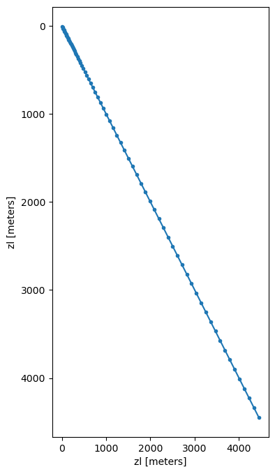
We can now access the horizontal and vertical grid of the regional configuration via expt.hgrid and expt.vgrid respectively.
Plotting the vertical grid with marker = '.' lets us see the spacing.
[9]:
expt.vgrid.zl.plot(marker='.',
                   y='zl',
                   yincrease=False,
                   figsize=(4, 8))
[9]:
[<matplotlib.lines.Line2D at 0x1537a683a410>]
Modular workflow!
After constructing our expt object, if we are not happy with the default horizontal and vertical grids, hgrid and vgrid, we can simply modify and then save them back into the expt object. However, we’ll then also need to save them to disk again. For example:
new_hgrid = xr.open_dataset(input_dir + "/hgrid.nc")
Modify new_hgrid, ensuring that all metadata is retained to keep MOM6 happy. Then, save our changes:
expt.hgrid = new_hgrid

expt.hgrid.to_netcdf(input_dir + "/hgrid.nc")
Step 4: Set up bathymetry
Similarly to ocean forcing, we point the experiment’s setup_bathymetry method at the location of the file of choice and also provide the variable names. We don’t need to preprocess the bathymetry since it is simply a two-dimensional field and is easier to deal with. Afterwards we can inspect expt.bathymetry to see our regional domain.
After running this cell, our input directory will contain other bathymetry-related things like the ocean mosaic and mask table too. The mask table defaults to a 10x10 layout and can be modified later.
[10]:
expt.setup_bathymetry(
    bathymetry_path='/g/data/ik11/inputs/GEBCO_2022/GEBCO_2022.nc',
    longitude_coordinate_name='lon',
    latitude_coordinate_name='lat',
    vertical_coordinate_name='elevation',
    )
INFO:regional_mom6.regridding:Getting t points..
INFO:regional_mom6.regridding:Creating Regridder
Begin regridding bathymetry...

Original bathymetry size: 37.08 Mb
Regridded size: 0.84 Mb
Automatic regridding may fail if your domain is too big! If this process hangs or crashes,make sure function argument write_to_file = True and,open a terminal with appropriate computational and resources try calling ESMF directly in the input directory /scratch/gb02/nc3020/regional_mom6_configs/tassie-access-om2-forced via

`mpirun -np NUMBER_OF_CPUS ESMF_Regrid -s bathymetry_original.nc -d bathymetry_unfinished.nc -m bilinear --src_var depth --dst_var depth --netcdf4 --src_regional --dst_regional`

For details see https://xesmf.readthedocs.io/en/latest/large_problems_on_HPC.html

Afterwards, we run the 'expt.tidy_bathymetry' method to skip the expensive interpolation step, and finishing metadata, encoding and cleanup.


Regridding successful! Now calling `tidy_bathymetry` method for some finishing touches...
setup bathymetry has finished successfully.
Tidy bathymetry: Reading in regridded bathymetry to fix up metadata...done. Filling in inland lakes and channels...
[10]:
<xarray.Dataset> Size: 837kB
Dimensions:  (ny: 249, nx: 140)
Coordinates:
    lon      (ny, nx) float64 279kB 143.0 143.1 143.1 ... 149.9 149.9 150.0
    lat      (ny, nx) float64 279kB -47.98 -47.98 -47.98 ... -38.97 -38.97
Dimensions without coordinates: ny, nx
Data variables:
    depth    (ny, nx) float64 279kB 4.584e+03 4.552e+03 ... 4.215e+03 4.364e+03
Attributes:
    depth:          meters
    standard_name:  bathymetric depth at T-cell centers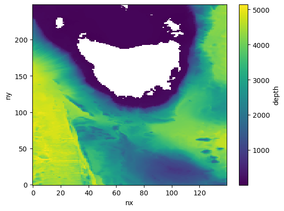
coordinates: ziCheck out our domain:
[11]:
expt.bathymetry.depth.plot()
[11]:
<matplotlib.collections.QuadMesh at 0x1537909a37d0>
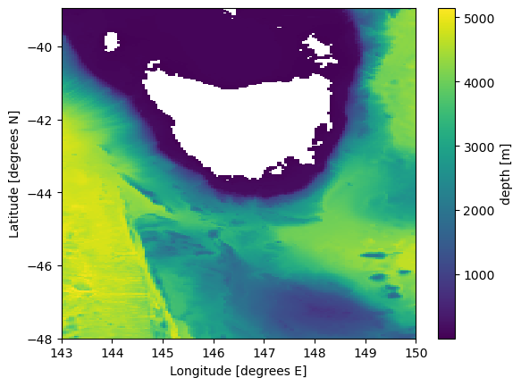
We can can add geographical coordinates to the plot above, e.g.,
[12]:
plt.pcolormesh(expt.bathymetry.lon, expt.bathymetry.lat, expt.bathymetry.depth[0, :, :], shading='auto')
plt.colorbar(label = 'depth [m]')
plt.xlabel('Longitude [degrees E]')
plt.ylabel('Latitude [degrees N]');
Step 5: Handle the ocean forcing - where the magic happens
This cuts out and interpolates the initial condition as well as all boundaries (unless we don’t pass it boundaries).
The dictionary maps the MOM6 variable names to what they’re called in our ocean input file. Notice how the horizontal dimensions are xt_ocean, yt_ocean, xu_ocean, yu_ocean in ACCESS-OM2-01 versus xh, yh, xq, and yq in MOM6. This is because ACCESS-OM2-01 is on a B grid, so we need to differentiate between q and t points.
If one of our segments is land, we can delete its string from the ‘boundaries’ list. We need to update MOM_input to reflect this though so that MOM6 knows how many segments to look for, and their orientations.
Define a mapping from the MOM5 B-grid variables and dimensions to the MOM6 C-grid ones.
[13]:
ocean_varnames = {"time": "time",
                  "yh": "yt_ocean",
                  "xh": "xt_ocean",
                  "xq": "xu_ocean",
                  "yq": "yu_ocean",
                  "zl": "st_ocean",
                  "eta": "eta_t",
                  "u": "u",
                  "v": "v",
                  "tracers": {"salt": "salt", "temp": "temp"}
                  }
Set up the initial condition
No xu_ocean and xt_ocean in west_unprocessed.nc and east_unprocessed.nc
xu_ocean = UNLIMITED ; // (0 currently)
[14]:
# Set up the initial condition.
expt.setup_initial_condition(
    tmp_dir + "/ic_unprocessed.nc", # directory where the unprocessed initial condition is stored, as defined earlier
    ocean_varnames,
    arakawa_grid = "B"
    )

# Set up the four boundary conditions.
expt.setup_ocean_state_boundaries(
    Path(tmp_dir),
    ocean_varnames,
    arakawa_grid = "B"
    )
INFO:regional_mom6.regridding:Getting t points..
INFO:regional_mom6.regridding:Creating Regridder
INFO:regional_mom6.regridding:Creating Regridder
INFO:regional_mom6.regridding:Creating Regridder
Setting up Initial Conditions
Regridding Velocities...
INFO:regional_mom6.rotation:Getting rotation angle
INFO:regional_mom6.rotation:Calculating grid rotation angle
INFO:regional_mom6.regridding:Getting u points..
INFO:regional_mom6.regridding:Getting v points..
Done.
Regridding Tracers... Done.
Regridding Free surface... Done.
Saving outputs...
INFO:regional_mom6.regridding:Creating coordinates of the boundary q/u/v points
INFO:regional_mom6.regridding:Creating Regridder
WARNING:regional_mom6.regridding:Using existing weights file at /scratch/gb02/nc3020/regional_mom6_configs/tassie-access-om2-forced/weights/bilinear_velocity_weights_north.nc to save computing time. Delete weights file to regenerate weights.
INFO:regional_mom6.regridding:Creating Regridder
WARNING:regional_mom6.regridding:Using existing weights file at /scratch/gb02/nc3020/regional_mom6_configs/tassie-access-om2-forced/weights/bilinear_tracer_weights_north.nc to save computing time. Delete weights file to regenerate weights.
done setting up initial condition.
Processing north boundary velocity & tracers...
INFO:regional_mom6.rotation:Getting rotation angle
INFO:regional_mom6.rotation:Calculating grid rotation angle
INFO:regional_mom6.regridding:Creating coordinates of the boundary q/u/v points
INFO:regional_mom6.regridding:Filling in missing data horizontally, then vertically
INFO:regional_mom6.regridding:Adding time dimension
INFO:regional_mom6.regridding:Renaming vertical coordinate to nz_... in salt_segment_001
INFO:regional_mom6.regridding:Replacing old depth coordinates with incremental integers
INFO:regional_mom6.regridding:Adding perpendicular dimension to salt_segment_001
INFO:regional_mom6.regridding:Renaming vertical coordinate to nz_... in temp_segment_001
INFO:regional_mom6.regridding:Replacing old depth coordinates with incremental integers
INFO:regional_mom6.regridding:Adding perpendicular dimension to temp_segment_001
INFO:regional_mom6.regridding:Renaming vertical coordinate to nz_... in u_segment_001
INFO:regional_mom6.regridding:Replacing old depth coordinates with incremental integers
INFO:regional_mom6.regridding:Adding perpendicular dimension to u_segment_001
INFO:regional_mom6.regridding:Renaming vertical coordinate to nz_... in v_segment_001
INFO:regional_mom6.regridding:Replacing old depth coordinates with incremental integers
INFO:regional_mom6.regridding:Adding perpendicular dimension to v_segment_001
INFO:regional_mom6.regridding:Adding perpendicular dimension to eta_segment_001
WARNING:regional_mom6.regridding:All NaNs filled b/c bathymetry wasn't provided to the function. Add bathymetry_path to the segment class to avoid this
INFO:regional_mom6.regridding:Generating encoding dictionary
INFO:regional_mom6.regridding:Creating coordinates of the boundary q/u/v points
INFO:regional_mom6.regridding:Creating Regridder
WARNING:regional_mom6.regridding:Using existing weights file at /scratch/gb02/nc3020/regional_mom6_configs/tassie-access-om2-forced/weights/bilinear_velocity_weights_south.nc to save computing time. Delete weights file to regenerate weights.
INFO:regional_mom6.regridding:Creating Regridder
WARNING:regional_mom6.regridding:Using existing weights file at /scratch/gb02/nc3020/regional_mom6_configs/tassie-access-om2-forced/weights/bilinear_tracer_weights_south.nc to save computing time. Delete weights file to regenerate weights.
INFO:regional_mom6.rotation:Getting rotation angle
INFO:regional_mom6.rotation:Calculating grid rotation angle
INFO:regional_mom6.regridding:Creating coordinates of the boundary q/u/v points
INFO:regional_mom6.regridding:Filling in missing data horizontally, then vertically
INFO:regional_mom6.regridding:Adding time dimension
INFO:regional_mom6.regridding:Renaming vertical coordinate to nz_... in salt_segment_002
INFO:regional_mom6.regridding:Replacing old depth coordinates with incremental integers
INFO:regional_mom6.regridding:Adding perpendicular dimension to salt_segment_002
INFO:regional_mom6.regridding:Renaming vertical coordinate to nz_... in temp_segment_002
INFO:regional_mom6.regridding:Replacing old depth coordinates with incremental integers
INFO:regional_mom6.regridding:Adding perpendicular dimension to temp_segment_002
INFO:regional_mom6.regridding:Renaming vertical coordinate to nz_... in u_segment_002
INFO:regional_mom6.regridding:Replacing old depth coordinates with incremental integers
INFO:regional_mom6.regridding:Adding perpendicular dimension to u_segment_002
INFO:regional_mom6.regridding:Renaming vertical coordinate to nz_... in v_segment_002
INFO:regional_mom6.regridding:Replacing old depth coordinates with incremental integers
INFO:regional_mom6.regridding:Adding perpendicular dimension to v_segment_002
INFO:regional_mom6.regridding:Adding perpendicular dimension to eta_segment_002
WARNING:regional_mom6.regridding:All NaNs filled b/c bathymetry wasn't provided to the function. Add bathymetry_path to the segment class to avoid this
Done.
Processing south boundary velocity & tracers...
INFO:regional_mom6.regridding:Generating encoding dictionary
INFO:regional_mom6.regridding:Creating coordinates of the boundary q/u/v points
INFO:regional_mom6.regridding:Creating Regridder
WARNING:regional_mom6.regridding:Using existing weights file at /scratch/gb02/nc3020/regional_mom6_configs/tassie-access-om2-forced/weights/bilinear_velocity_weights_east.nc to save computing time. Delete weights file to regenerate weights.
INFO:regional_mom6.regridding:Creating Regridder
WARNING:regional_mom6.regridding:Using existing weights file at /scratch/gb02/nc3020/regional_mom6_configs/tassie-access-om2-forced/weights/bilinear_tracer_weights_east.nc to save computing time. Delete weights file to regenerate weights.
INFO:regional_mom6.rotation:Getting rotation angle
INFO:regional_mom6.rotation:Calculating grid rotation angle
INFO:regional_mom6.regridding:Creating coordinates of the boundary q/u/v points
INFO:regional_mom6.regridding:Filling in missing data horizontally, then vertically
INFO:regional_mom6.regridding:Adding time dimension
INFO:regional_mom6.regridding:Renaming vertical coordinate to nz_... in salt_segment_003
INFO:regional_mom6.regridding:Replacing old depth coordinates with incremental integers
INFO:regional_mom6.regridding:Adding perpendicular dimension to salt_segment_003
INFO:regional_mom6.regridding:Renaming vertical coordinate to nz_... in temp_segment_003
INFO:regional_mom6.regridding:Replacing old depth coordinates with incremental integers
INFO:regional_mom6.regridding:Adding perpendicular dimension to temp_segment_003
INFO:regional_mom6.regridding:Renaming vertical coordinate to nz_... in u_segment_003
INFO:regional_mom6.regridding:Replacing old depth coordinates with incremental integers
INFO:regional_mom6.regridding:Adding perpendicular dimension to u_segment_003
INFO:regional_mom6.regridding:Renaming vertical coordinate to nz_... in v_segment_003
INFO:regional_mom6.regridding:Replacing old depth coordinates with incremental integers
INFO:regional_mom6.regridding:Adding perpendicular dimension to v_segment_003
INFO:regional_mom6.regridding:Adding perpendicular dimension to eta_segment_003
WARNING:regional_mom6.regridding:All NaNs filled b/c bathymetry wasn't provided to the function. Add bathymetry_path to the segment class to avoid this
Done.
Processing east boundary velocity & tracers...
INFO:regional_mom6.regridding:Generating encoding dictionary
INFO:regional_mom6.regridding:Creating coordinates of the boundary q/u/v points
INFO:regional_mom6.regridding:Creating Regridder
WARNING:regional_mom6.regridding:Using existing weights file at /scratch/gb02/nc3020/regional_mom6_configs/tassie-access-om2-forced/weights/bilinear_velocity_weights_west.nc to save computing time. Delete weights file to regenerate weights.
INFO:regional_mom6.regridding:Creating Regridder
WARNING:regional_mom6.regridding:Using existing weights file at /scratch/gb02/nc3020/regional_mom6_configs/tassie-access-om2-forced/weights/bilinear_tracer_weights_west.nc to save computing time. Delete weights file to regenerate weights.
INFO:regional_mom6.rotation:Getting rotation angle
INFO:regional_mom6.rotation:Calculating grid rotation angle
INFO:regional_mom6.regridding:Creating coordinates of the boundary q/u/v points
INFO:regional_mom6.regridding:Filling in missing data horizontally, then vertically
INFO:regional_mom6.regridding:Adding time dimension
Done.
Processing west boundary velocity & tracers...
INFO:regional_mom6.regridding:Renaming vertical coordinate to nz_... in salt_segment_004
INFO:regional_mom6.regridding:Replacing old depth coordinates with incremental integers
INFO:regional_mom6.regridding:Adding perpendicular dimension to salt_segment_004
INFO:regional_mom6.regridding:Renaming vertical coordinate to nz_... in temp_segment_004
INFO:regional_mom6.regridding:Replacing old depth coordinates with incremental integers
INFO:regional_mom6.regridding:Adding perpendicular dimension to temp_segment_004
INFO:regional_mom6.regridding:Renaming vertical coordinate to nz_... in u_segment_004
INFO:regional_mom6.regridding:Replacing old depth coordinates with incremental integers
INFO:regional_mom6.regridding:Adding perpendicular dimension to u_segment_004
INFO:regional_mom6.regridding:Renaming vertical coordinate to nz_... in v_segment_004
INFO:regional_mom6.regridding:Replacing old depth coordinates with incremental integers
INFO:regional_mom6.regridding:Adding perpendicular dimension to v_segment_004
INFO:regional_mom6.regridding:Adding perpendicular dimension to eta_segment_004
WARNING:regional_mom6.regridding:All NaNs filled b/c bathymetry wasn't provided to the function. Add bathymetry_path to the segment class to avoid this
INFO:regional_mom6.regridding:Generating encoding dictionary
Done.
We can inspect all variable in the experiment by calling
[15]:
vars(expt)
[15]:
{'expt_name': None,
 'date_range': [datetime.datetime(2013, 1, 1, 0, 0),
  datetime.datetime(2013, 1, 5, 0, 0)],
 'mom_run_dir': PosixPath('/home/552/nc3020/mom6_rundirs/tassie-access-om2-forced'),
 'mom_input_dir': PosixPath('/scratch/gb02/nc3020/regional_mom6_configs/tassie-access-om2-forced'),
 'fre_tools_dir': PosixPath('/g/data/ik11/mom6_tools/tools'),
 'resolution': 0.05,
 'number_vertical_layers': 75,
 'layer_thickness_ratio': 10,
 'depth': 4500,
 'hgrid_type': 'even_spacing',
 'vgrid_type': 'hyperbolic_tangent',
 'repeat_year_forcing': False,
 'ocean_mask': <xarray.DataArray 'depth' (ny: 249, nx: 140)> Size: 279kB
 array([[1, 1, 1, ..., 1, 1, 1],
        [1, 1, 1, ..., 1, 1, 1],
        [1, 1, 1, ..., 1, 1, 1],
        ...,
        [1, 1, 1, ..., 1, 1, 1],
        [1, 1, 1, ..., 1, 1, 1],
        [1, 1, 1, ..., 1, 1, 1]])
 Coordinates:
     lon      (ny, nx) float64 279kB 143.0 143.1 143.1 ... 149.9 149.9 150.0
     lat      (ny, nx) float64 279kB -47.98 -47.98 -47.98 ... -38.97 -38.97
 Dimensions without coordinates: ny, nx,
 'layout': None,
 'minimum_depth': 4,
 'tidal_constituents': ['M2',
  'S2',
  'N2',
  'K2',
  'K1',
  'O1',
  'P1',
  'Q1',
  'MM',
  'MF'],
 'regridding_method': 'bilinear',
 'fill_method': <function regional_mom6.regridding.fill_missing_data(ds: xarray.core.dataset.Dataset, xdim: str = 'locations', zdim: str = 'z', fill: str = 'b') -> xarray.core.dataset.Dataset>,
 'longitude_extent': (143, 150),
 'latitude_extent': (-48, -38.95),
 'hgrid': <xarray.Dataset> Size: 10MB
 Dimensions:       (nyp: 499, nxp: 281, nx: 280, ny: 498)
 Coordinates:
   * nyp           (nyp) int64 4kB 0 1 2 3 4 5 6 ... 492 493 494 495 496 497 498
   * nxp           (nxp) int64 2kB 0 1 2 3 4 5 6 ... 274 275 276 277 278 279 280
 Dimensions without coordinates: nx, ny
 Data variables:
     tile          |S255 255B b'tile1'
     x             (nyp, nxp) float64 1MB 143.0 143.0 143.1 ... 149.9 150.0 150.0
     y             (nyp, nxp) float64 1MB -48.0 -48.0 -48.0 ... -38.95 -38.95
     dx            (nyp, nx) float64 1MB 930.0 930.0 ... 1.081e+03 1.081e+03
     dy            (ny, nxp) float64 1MB 1.01e+03 1.01e+03 ... 1.01e+03 1.01e+03
     area          (ny, nx) float64 1MB 3.759e+06 3.759e+06 ... 4.368e+06
     angle_dx      (nyp, nxp) float64 1MB 0.0 0.0 0.0 0.0 0.0 ... 0.0 0.0 0.0 0.0
     arcx          |S255 255B b'small_circle'
     lon           (nyp, nxp) float64 1MB 143.0 143.0 143.1 ... 149.9 150.0 150.0
     lat           (nyp, nxp) float64 1MB -48.0 -48.0 -48.0 ... -38.95 -38.95
     angle_dx_rm6  (nyp, nxp) float64 1MB -0.0 -0.0 -0.0 -0.0 ... -0.0 -0.0 -0.0,
 'vgrid': <xarray.Dataset> Size: 1kB
 Dimensions:  (zi: 76, zl: 75)
 Coordinates:
   * zi       (zi) float64 608B 0.0 11.09 22.22 ... 4.282e+03 4.391e+03 4.5e+03
   * zl       (zl) float64 600B 5.546 16.66 27.8 ... 4.337e+03 4.446e+03
 Data variables:
     *empty*,
 'segments': {'north': <regional_mom6.regional_mom6.segment at 0x153791a74990>,
  'south': <regional_mom6.regional_mom6.segment at 0x1537903ba490>,
  'east': <regional_mom6.regional_mom6.segment at 0x1537a5082e90>,
  'west': <regional_mom6.regional_mom6.segment at 0x1537903c8e50>},
 'boundaries': ['north', 'south', 'east', 'west'],
 'ic_eta': <xarray.DataArray 'eta_t' (ny: 249, nx: 140)> Size: 139kB
 dask.array<astype, shape=(249, 140), dtype=float32, chunksize=(249, 140), chunktype=numpy.ndarray>
 Coordinates:
     xh       (ny, nx) float64 279kB 143.0 143.1 143.1 ... 149.9 149.9 150.0
     yh       (ny, nx) float64 279kB -47.98 -47.98 -47.98 ... -38.97 -38.97
 Dimensions without coordinates: ny, nx
 Attributes:
     time_avg_info:  average_T1,average_T2,average_DT
     long_name:      surface height on T cells [Boussinesq (volume conserving)...
     cell_methods:   time: mean
     units:          meter
     valid_range:    [-1000.  1000.],
 'ic_tracers': <xarray.Dataset> Size: 21MB
 Dimensions:  (ny: 249, nx: 140, zl: 75)
 Coordinates:
     xh       (ny, nx) float64 279kB 143.0 143.1 143.1 ... 149.9 149.9 150.0
     yh       (ny, nx) float64 279kB -47.98 -47.98 -47.98 ... -38.97 -38.97
   * nx       (nx) float64 1kB 0.0 1.0 2.0 3.0 4.0 ... 136.0 137.0 138.0 139.0
   * ny       (ny) float64 2kB 0.0 1.0 2.0 3.0 4.0 ... 245.0 246.0 247.0 248.0
   * zl       (zl) float64 600B 5.546 16.66 27.8 ... 4.337e+03 4.446e+03
 Data variables:
     salt     (zl, ny, nx) float32 10MB dask.array<chunksize=(75, 249, 140), meta=np.ndarray>
     temp     (zl, ny, nx) float32 10MB dask.array<chunksize=(75, 249, 140), meta=np.ndarray>
 Attributes:
     regrid_method:  bilinear,
 'ic_vels': <xarray.Dataset> Size: 43MB
 Dimensions:  (ny: 249, nxp: 141, zl: 75, nyp: 250, nx: 140)
 Coordinates:
   * ny       (ny) int64 2kB 1 3 5 7 9 11 13 15 ... 485 487 489 491 493 495 497
   * nxp      (nxp) int64 1kB 0 2 4 6 8 10 12 14 ... 268 270 272 274 276 278 280
     xq       (ny, nxp) float64 281kB 143.0 143.1 143.1 ... 149.9 149.9 150.0
     yh       (ny, nxp) float64 281kB -47.98 -47.98 -47.98 ... -38.97 -38.97
   * nyp      (nyp) int64 2kB 0 2 4 6 8 10 12 14 ... 486 488 490 492 494 496 498
   * nx       (nx) int64 1kB 1 3 5 7 9 11 13 15 ... 267 269 271 273 275 277 279
     xh       (nyp, nx) float64 280kB 143.0 143.1 143.1 ... 149.9 149.9 150.0
     yq       (nyp, nx) float64 280kB -48.0 -48.0 -48.0 ... -38.95 -38.95 -38.95
   * zl       (zl) float64 600B 5.546 16.66 27.8 ... 4.337e+03 4.446e+03
 Data variables:
     u        (zl, ny, nxp) float64 21MB dask.array<chunksize=(75, 249, 141), meta=np.ndarray>
     v        (zl, nyp, nx) float64 21MB dask.array<chunksize=(75, 250, 140), meta=np.ndarray>}
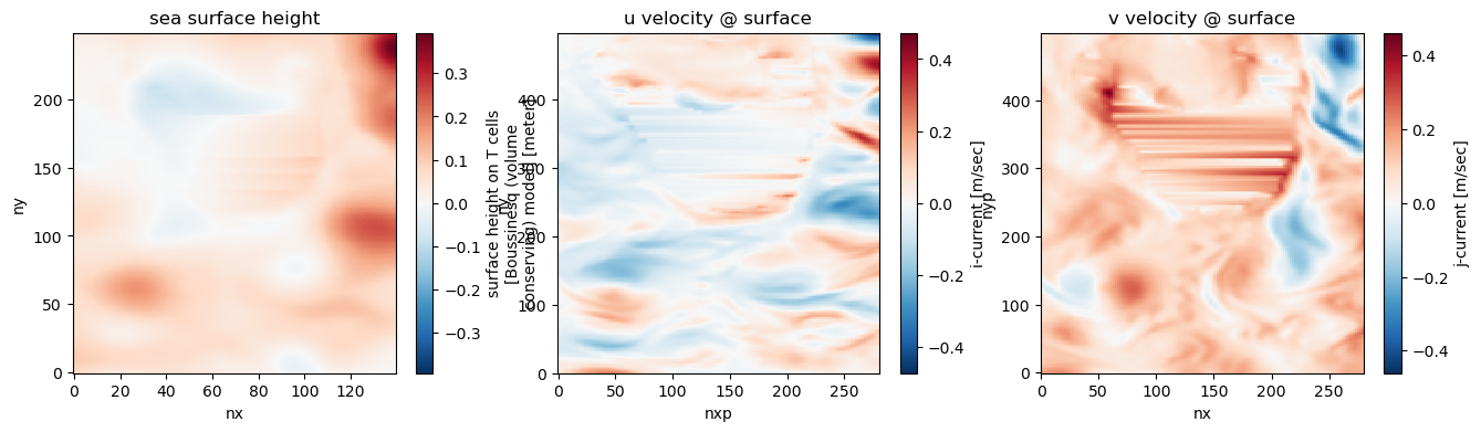
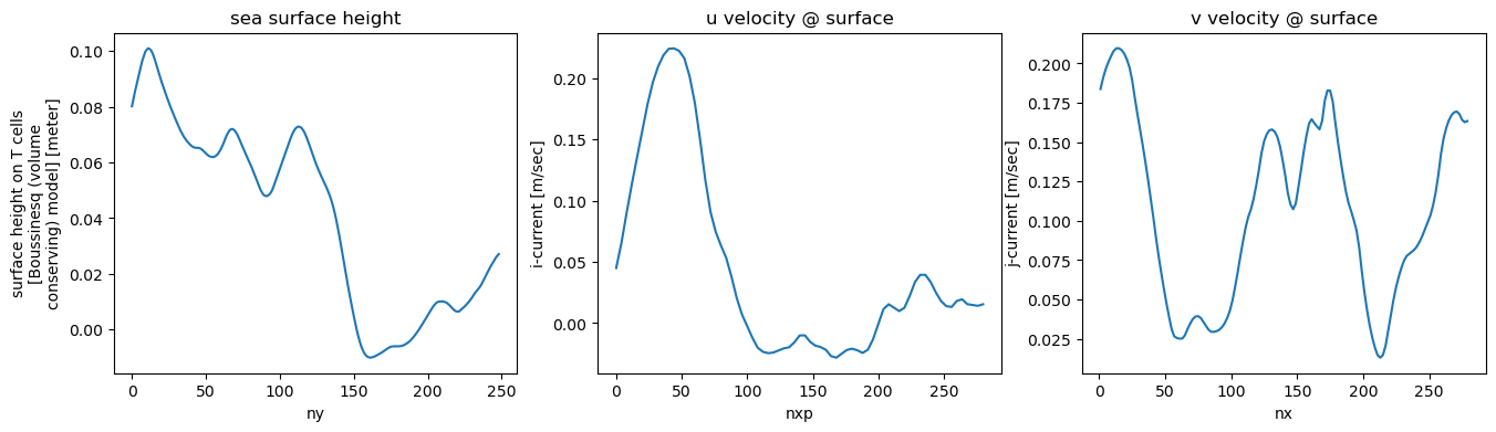
Furthermore, we can plot our the interpolated initial condition. It’s a good idea to check and ensure things look reasonble, especially near the region’s boundaries.
[16]:
fig, axes = plt.subplots(ncols=3, figsize=(16, 4))

expt.ic_eta.plot(ax=axes[0])
expt.ic_vels.u.sel(zl=0, method='nearest').plot(ax=axes[1])
expt.ic_vels.v.sel(zl=0, method='nearest').plot(ax=axes[2])

axes[0].set_title("sea surface height")
axes[1].set_title("u velocity @ surface")
axes[2].set_title("v velocity @ surface");
To ensure that no spurious gradients have emerged at the boundaries (e.g., during the interpolation) we plot a few slices, e.g.,
[17]:
fig, axes = plt.subplots(ncols=3, figsize=(16, 4))

expt.ic_eta.isel(nx=0).plot(ax=axes[0])
expt.ic_vels.u.isel(ny=0, zl=0).plot(ax=axes[1])
expt.ic_vels.v.isel(nyp=0, zl=0).plot(ax=axes[2])

axes[0].set_title("sea surface height")
axes[1].set_title("u velocity @ surface")
axes[2].set_title("v velocity @ surface");
Step 6: Run the FRE tools
This is just a wrapper for the FRE tools needed to make the mosaics and masks for the experiment. The only thing we need to tell it is the processor layout. In this case we’re asking for a 10 by 10 grid of 100 processors.
[18]:
expt.run_FRE_tools(layout = (10, 10)) ## tuple defines the processor layout
Running GFDL's FRE Tools. The following information is all printed by the FRE tools themselves
NOTE from make_solo_mosaic: there are 0 contacts (align-contact)
congradulation: You have successfully run make_solo_mosaic
OUTPUT FROM MAKE SOLO MOSAIC:

CompletedProcess(args='/g/data/ik11/mom6_tools/tools/make_solo_mosaic/make_solo_mosaic --num_tiles 1 --dir . --mosaic_name ocean_mosaic --tile_file hgrid.nc', returncode=0)
cp: './ocean_mosaic.nc' and 'ocean_mosaic.nc' are the same file
cp: './hgrid.nc' and 'hgrid.nc' are the same file
cp ./hgrid.nc hgrid.nc

NOTE from make_coupler_mosaic: the ocean land/sea mask will be determined by field depth from file bathymetry.nc
mosaic_file is grid_spec.nc

***** Congratulation! You have successfully run make_quick_mosaic
OUTPUT FROM QUICK MOSAIC:

CompletedProcess(args='/g/data/ik11/mom6_tools/tools/make_quick_mosaic/make_quick_mosaic --input_mosaic ocean_mosaic.nc --mosaic_name grid_spec --ocean_topog bathymetry.nc', returncode=0)

 ===>NOTE from check_mask: when layout is specified, min_pe and max_pe is set to layout(1)*layout(2)=100

 ===>NOTE from check_mask: Below is the list of command line arguments.

grid_file = ocean_mosaic.nc
topog_file = bathymetry.nc
min_pe = 100
max_pe = 100
layout = 10, 10
halo = 4
sea_level = 0
show_valid_only is not set
nobc = 0

 ===>NOTE from check_mask: End of command line arguments.

 ===>NOTE from check_mask: the grid file is version 2 (mosaic grid) grid which contains field gridfiles

==>NOTE from get_boundary_type: x_boundary_type is solid_walls

==>NOTE from get_boundary_type: y_boundary_type is solid_walls

==>NOTE from check_mask: Checking for possible masking:
==>NOTE from check_mask: Assume 4 halo rows
==>NOTE from check_mask: Total domain size is 140, 249

_______________________________________________________________________

NOTE from check_mask: The following is for using model source code with version older than siena_201207,
Possible setting to mask out all-land points region, for use in coupler_nmlTotal number of domains = 100
Number of tasks (excluded all-land region) to be used is 98
Number of regions to be masked out = 2
The layout is 10, 10
Masked and used tasks, 1: used, 0: masked
1111111111
1111111111
1111111111
1111001111
1111111111
1111111111
1111111111
1111111111
1111111111
1111111111
 domain decomposition
  14  14  14  14  14  14  14  14  14  14
  25  25  25  25  25  25  25  25  25  24
 used=98, masked=2, layout=10,10
 To chose this mask layout please put the following lines in ocean_model_nml and/or ice_model_nml
 nmask = 2
layout = 10, 10
mask_list = 5,7,6,7


_______________________________________________________________________

NOTE from check_mask: The following is for using model source code with version siena_201207 or newer,
                      specify ocean_model_nml/ice_model_nml/atmos_model_nml/land_model/nml
                      variable mask_table with the mask_table created here.
                      Also specify the layout variable in each namelist using corresponding layout

***** Congratulation! You have successfully run check_mask
OUTPUT FROM CHECK MASK:

 CompletedProcess(args='/g/data/ik11/mom6_tools/tools/check_mask/check_mask --grid_file ocean_mosaic.nc --ocean_topog bathymetry.nc --layout 10,10 --halo 4', returncode=0)
Step 7: Modify the default input directory to make a runnable configuration out of the box
This step copies the default directory, and modifies the MOM_layout files to match your experiment by inserting the right number of x, y points and the CPU layout. If we use payu to run MOM6, then we set the using_payu flag to True. This way, an example config.yaml file is copied to our run directory. This config.yaml still needs to be modified manually to add our NCI projets, locations of executable, etc.
[19]:
expt.setup_run_directory(surface_forcing = "jra", using_payu = True)
Mask table mask_table.2.10x10 read. Using this to infer the cpu layout (10, 10), total masked out cells 2, and total number of CPUs 98.
Deleting indexed OBC keys from MOM_input_dict in case we have a different number of segments
Step 8: Run your model!
To do this, we navigate to our run directory in terminal. If we are working on NCI, we can run our model via:
module load conda/analysis3
payu setup -f
payu run -f
By default input.nml is set to only run for 5 days as a test. If this is successful, then we can modify this file to run for longer.
Step 9 and beyond: Fiddling, troubleshooting, and fine tuning
Hopefully our model is running. If not, the first thing we should do is reduce the timestep. We can do this by adding #override DT=XXXX to your MOM_override file.
If there’s strange behaviour on our boundaries, we can play around with the nudging timescale (an example is already included in the MOM_override file). Sometimes, if a boundary has a lot going on (like all of the eddies spinning off the western boundary currents or off the Antarctic Circumpolar current), it can be hard to avoid these edge effects. This is because the chaotic, submesoscale structures developed within the regional domain won’t match those at the boundary.
Another thing that can go wrong is little bays creating non-advective cells at your boundaries. Keep an eye out for tiny bays where one side is taken up by a boundary segment. We can either fill them in manually, or move your boundary slightly to avoid them.
[20]:
client.close()