Horizontal regridding and comparing different resolutions
This notebook demonstrates regridding the ACCESS-OM2 output onto a different grid. In this example, regridding model output from all three ACCESS-OM2 resolutions on to a 1-degree longitude-latitude grid with regular spacing.
Requirements: This notebook has been tested using the conda/analysis3-26.06 module on ARE/gadi
Conversion to MOM6:
MOM6 uses a different grid to MOM5/ACCESS-OM2, so be aware of the differences when doing regridding of velocity or transport variables which are positioned differently on the grid to MOM5. However, sea surface height also lives on the h or tracer grid, so this recipe could be converted to MOM6 with the following variable changes.
MOM5 variable |
MOM6 variable |
|---|---|
|
|
|
|
|
|
|
|
|
|
|
|
|
|
Firstly, load in the requisite libraries:
[1]:
import intake

import matplotlib.pyplot as plt
import cartopy.crs as ccrs

import xarray as xr

xr.set_options(keep_attrs=True)

from dask.distributed import Client

import xesmf
Load a dask client. This is not required for small regridding jobs, and does not affect the speed of generating the regridding weights, but may improve speed, or reduce memory overhead, when regridding large datasets with, for example, large time dimensions.
[2]:
client = Client(threads_per_worker=1)
client
[2]:
Client
Client-831b10a7-75a6-11f1-bead-000003f5fe80
| Connection method: Cluster object | Cluster type: distributed.LocalCluster |
| Dashboard: /proxy/8787/status |
Cluster Info
LocalCluster
308e3474
| Dashboard: /proxy/8787/status | Workers: 28 |
| Total threads: 28 | Total memory: 251.19 GiB |
| Status: running | Using processes: True |
Scheduler Info
Scheduler
Scheduler-92e41cf9-c390-47c0-a871-48588416a0ae
| Comm: tcp://127.0.0.1:44949 | Workers: 0 |
| Dashboard: /proxy/8787/status | Total threads: 0 |
| Started: Just now | Total memory: 0 B |
Workers
Worker: 0
| Comm: tcp://127.0.0.1:35643 | Total threads: 1 |
| Dashboard: /proxy/39433/status | Memory: 8.97 GiB |
| Nanny: tcp://127.0.0.1:38507 | |
| Local directory: /jobfs/172823967.gadi-pbs/dask-scratch-space/worker-4v_r0cgk | |
Worker: 1
| Comm: tcp://127.0.0.1:33983 | Total threads: 1 |
| Dashboard: /proxy/44697/status | Memory: 8.97 GiB |
| Nanny: tcp://127.0.0.1:45525 | |
| Local directory: /jobfs/172823967.gadi-pbs/dask-scratch-space/worker-3c6wjlg6 | |
Worker: 2
| Comm: tcp://127.0.0.1:43855 | Total threads: 1 |
| Dashboard: /proxy/36149/status | Memory: 8.97 GiB |
| Nanny: tcp://127.0.0.1:33725 | |
| Local directory: /jobfs/172823967.gadi-pbs/dask-scratch-space/worker-i_674l9l | |
Worker: 3
| Comm: tcp://127.0.0.1:36451 | Total threads: 1 |
| Dashboard: /proxy/38881/status | Memory: 8.97 GiB |
| Nanny: tcp://127.0.0.1:42891 | |
| Local directory: /jobfs/172823967.gadi-pbs/dask-scratch-space/worker-aapjvat9 | |
Worker: 4
| Comm: tcp://127.0.0.1:36583 | Total threads: 1 |
| Dashboard: /proxy/34779/status | Memory: 8.97 GiB |
| Nanny: tcp://127.0.0.1:46115 | |
| Local directory: /jobfs/172823967.gadi-pbs/dask-scratch-space/worker-6tge5zc0 | |
Worker: 5
| Comm: tcp://127.0.0.1:34047 | Total threads: 1 |
| Dashboard: /proxy/39213/status | Memory: 8.97 GiB |
| Nanny: tcp://127.0.0.1:37589 | |
| Local directory: /jobfs/172823967.gadi-pbs/dask-scratch-space/worker-59fcuhkh | |
Worker: 6
| Comm: tcp://127.0.0.1:41205 | Total threads: 1 |
| Dashboard: /proxy/45447/status | Memory: 8.97 GiB |
| Nanny: tcp://127.0.0.1:44667 | |
| Local directory: /jobfs/172823967.gadi-pbs/dask-scratch-space/worker-kmy3wm__ | |
Worker: 7
| Comm: tcp://127.0.0.1:36183 | Total threads: 1 |
| Dashboard: /proxy/36595/status | Memory: 8.97 GiB |
| Nanny: tcp://127.0.0.1:34147 | |
| Local directory: /jobfs/172823967.gadi-pbs/dask-scratch-space/worker-gcwpco8i | |
Worker: 8
| Comm: tcp://127.0.0.1:40833 | Total threads: 1 |
| Dashboard: /proxy/38071/status | Memory: 8.97 GiB |
| Nanny: tcp://127.0.0.1:40201 | |
| Local directory: /jobfs/172823967.gadi-pbs/dask-scratch-space/worker-n56s0_zw | |
Worker: 9
| Comm: tcp://127.0.0.1:44207 | Total threads: 1 |
| Dashboard: /proxy/36835/status | Memory: 8.97 GiB |
| Nanny: tcp://127.0.0.1:41475 | |
| Local directory: /jobfs/172823967.gadi-pbs/dask-scratch-space/worker-075d8mdw | |
Worker: 10
| Comm: tcp://127.0.0.1:45921 | Total threads: 1 |
| Dashboard: /proxy/40555/status | Memory: 8.97 GiB |
| Nanny: tcp://127.0.0.1:38333 | |
| Local directory: /jobfs/172823967.gadi-pbs/dask-scratch-space/worker-4mlsy1jg | |
Worker: 11
| Comm: tcp://127.0.0.1:34091 | Total threads: 1 |
| Dashboard: /proxy/37737/status | Memory: 8.97 GiB |
| Nanny: tcp://127.0.0.1:35457 | |
| Local directory: /jobfs/172823967.gadi-pbs/dask-scratch-space/worker-m4ffzc47 | |
Worker: 12
| Comm: tcp://127.0.0.1:36865 | Total threads: 1 |
| Dashboard: /proxy/42213/status | Memory: 8.97 GiB |
| Nanny: tcp://127.0.0.1:37065 | |
| Local directory: /jobfs/172823967.gadi-pbs/dask-scratch-space/worker-vzugf_dv | |
Worker: 13
| Comm: tcp://127.0.0.1:44871 | Total threads: 1 |
| Dashboard: /proxy/35431/status | Memory: 8.97 GiB |
| Nanny: tcp://127.0.0.1:41257 | |
| Local directory: /jobfs/172823967.gadi-pbs/dask-scratch-space/worker-27vg0sip | |
Worker: 14
| Comm: tcp://127.0.0.1:37245 | Total threads: 1 |
| Dashboard: /proxy/37199/status | Memory: 8.97 GiB |
| Nanny: tcp://127.0.0.1:39289 | |
| Local directory: /jobfs/172823967.gadi-pbs/dask-scratch-space/worker-xawuqfg1 | |
Worker: 15
| Comm: tcp://127.0.0.1:41715 | Total threads: 1 |
| Dashboard: /proxy/42437/status | Memory: 8.97 GiB |
| Nanny: tcp://127.0.0.1:42651 | |
| Local directory: /jobfs/172823967.gadi-pbs/dask-scratch-space/worker-s9jy9zsr | |
Worker: 16
| Comm: tcp://127.0.0.1:38497 | Total threads: 1 |
| Dashboard: /proxy/44039/status | Memory: 8.97 GiB |
| Nanny: tcp://127.0.0.1:38915 | |
| Local directory: /jobfs/172823967.gadi-pbs/dask-scratch-space/worker-9sj7p07j | |
Worker: 17
| Comm: tcp://127.0.0.1:37119 | Total threads: 1 |
| Dashboard: /proxy/38409/status | Memory: 8.97 GiB |
| Nanny: tcp://127.0.0.1:34575 | |
| Local directory: /jobfs/172823967.gadi-pbs/dask-scratch-space/worker-6bc8ppsz | |
Worker: 18
| Comm: tcp://127.0.0.1:39021 | Total threads: 1 |
| Dashboard: /proxy/35585/status | Memory: 8.97 GiB |
| Nanny: tcp://127.0.0.1:40801 | |
| Local directory: /jobfs/172823967.gadi-pbs/dask-scratch-space/worker-o47md8j3 | |
Worker: 19
| Comm: tcp://127.0.0.1:42811 | Total threads: 1 |
| Dashboard: /proxy/39935/status | Memory: 8.97 GiB |
| Nanny: tcp://127.0.0.1:37367 | |
| Local directory: /jobfs/172823967.gadi-pbs/dask-scratch-space/worker-4esi61zv | |
Worker: 20
| Comm: tcp://127.0.0.1:39189 | Total threads: 1 |
| Dashboard: /proxy/36803/status | Memory: 8.97 GiB |
| Nanny: tcp://127.0.0.1:44099 | |
| Local directory: /jobfs/172823967.gadi-pbs/dask-scratch-space/worker-jqg85b9m | |
Worker: 21
| Comm: tcp://127.0.0.1:35687 | Total threads: 1 |
| Dashboard: /proxy/42151/status | Memory: 8.97 GiB |
| Nanny: tcp://127.0.0.1:36725 | |
| Local directory: /jobfs/172823967.gadi-pbs/dask-scratch-space/worker-qmn8sa8s | |
Worker: 22
| Comm: tcp://127.0.0.1:37611 | Total threads: 1 |
| Dashboard: /proxy/37551/status | Memory: 8.97 GiB |
| Nanny: tcp://127.0.0.1:44521 | |
| Local directory: /jobfs/172823967.gadi-pbs/dask-scratch-space/worker-k5hdqt56 | |
Worker: 23
| Comm: tcp://127.0.0.1:34695 | Total threads: 1 |
| Dashboard: /proxy/42989/status | Memory: 8.97 GiB |
| Nanny: tcp://127.0.0.1:34215 | |
| Local directory: /jobfs/172823967.gadi-pbs/dask-scratch-space/worker-0nxan28c | |
Worker: 24
| Comm: tcp://127.0.0.1:40823 | Total threads: 1 |
| Dashboard: /proxy/46457/status | Memory: 8.97 GiB |
| Nanny: tcp://127.0.0.1:41773 | |
| Local directory: /jobfs/172823967.gadi-pbs/dask-scratch-space/worker-q7wshupm | |
Worker: 25
| Comm: tcp://127.0.0.1:34129 | Total threads: 1 |
| Dashboard: /proxy/41611/status | Memory: 8.97 GiB |
| Nanny: tcp://127.0.0.1:35355 | |
| Local directory: /jobfs/172823967.gadi-pbs/dask-scratch-space/worker-kkqlvrt1 | |
Worker: 26
| Comm: tcp://127.0.0.1:34277 | Total threads: 1 |
| Dashboard: /proxy/37607/status | Memory: 8.97 GiB |
| Nanny: tcp://127.0.0.1:46535 | |
| Local directory: /jobfs/172823967.gadi-pbs/dask-scratch-space/worker-yy0nohf1 | |
Worker: 27
| Comm: tcp://127.0.0.1:43935 | Total threads: 1 |
| Dashboard: /proxy/40221/status | Memory: 8.97 GiB |
| Nanny: tcp://127.0.0.1:44313 | |
| Local directory: /jobfs/172823967.gadi-pbs/dask-scratch-space/worker-ol64ezc4 | |
Load a catalog; here we load the default ACCESS-NRI catalog.
[3]:
catalog = intake.cat.access_nri
Load raw data
We load some raw data from ACCESS-OM2 models. In particular, we load here the 2 years of monthly sea-surface height from the inter-annually forced ocean model runs at three different resolutions. These experiments are part of the default database and are called:
1deg_jra55_iaf_omip2_cycle6for ACCESS-OM2 1\(^\circ\) degree,025deg_jra55_iaf_omip2_cycle6for ACCESS-OM2 0.25\(^\circ\) degree,01deg_jra55v140_iaf_cycle4for ACCESS-OM2 0.1\(^\circ\) degree.
We use the intake catalog to load our variables.
We make sure to assign the correct tripolar coordinates as coords. Since sea-surface height is lives on t-cells, we add geolon_t and geolat_t. We also rename them to longitude and latitude to ease our life further down (xesmf package that we will use for regridding automatically searches for coordinates named longitude and latitude.)
After we load the data we rechunk them according to how the regridder’s needs; read further down for more details on this.
First, we load the grid parameters for each resolution.
[4]:
grid1 = intake.cat.access_nri["1deg_jra55_iaf_omip2_cycle6"].search(
    variable = ["geolat_t", "geolon_t", "geolat_c", "geolon_c"], frequency = "fx").to_dask()
grid025 = intake.cat.access_nri["025deg_jra55_iaf_omip2_cycle6"].search(
    variable = ["geolat_t", "geolon_t", "geolat_c", "geolon_c"], frequency = "fx").to_dask()

# for the 0.1deg model they are in different files
geolat_t01 = intake.cat.access_nri["01deg_jra55v140_iaf_cycle4"].search(
    variable = "geolat_t", frequency = "fx").to_dask()
geolon_t01 = intake.cat.access_nri["01deg_jra55v140_iaf_cycle4"].search(
    variable = "geolon_t", frequency = "fx").to_dask()
geolat_c01 = intake.cat.access_nri["01deg_jra55v140_iaf_cycle4"].search(
    variable = "geolat_c", frequency = "fx").to_dask()
geolon_c01 = intake.cat.access_nri["01deg_jra55v140_iaf_cycle4"].search(
    variable = "geolon_c", frequency = "fx").to_dask()
grid010 = xr.merge([geolat_t01,geolon_t01,geolat_c01,geolon_c01])
/jobfs/172757805.gadi-pbs/ipykernel_3610966/318327258.py:1: UserWarning: Value aliasing: variable='['geolat_t', 'geolon_t', 'geolat_c', 'geolon_c']' → variable=['c', 'geolat_t', 'l', 'g', 't', 'geolat_c', 'a', 'n', 'e', '_', 'o', 'geolon_c', 'geolon_t']
  grid1 = intake.cat.access_nri["1deg_jra55_iaf_omip2_cycle6"].search(
/jobfs/172757805.gadi-pbs/ipykernel_3610966/318327258.py:3: UserWarning: Value aliasing: variable='['geolat_t', 'geolon_t', 'geolat_c', 'geolon_c']' → variable=['c', 'geolat_t', 'l', 'g', 't', 'geolat_c', 'a', 'n', 'e', '_', 'o', 'geolon_c', 'geolon_t']
  grid025 = intake.cat.access_nri["025deg_jra55_iaf_omip2_cycle6"].search(
Now, we load the sea level variable for each resolution.
[5]:
ds = (
    catalog["1deg_jra55_iaf_omip2_cycle6"]
    .search(variable="sea_level", frequency="1mon")
    .to_dask()
)

ssh_1 = (
    ds["sea_level"]
    .sel(time=slice("2000-01-01", "2001-12-31"))
    .chunk({"time": "auto", "xt_ocean": -1, "yt_ocean": -1})
)
ssh_1 = ssh_1.assign_coords({"geolat_t": grid1.geolat_t, "geolon_t": grid1.geolon_t})
ssh_1 = ssh_1.rename({"xt_ocean": "x", "yt_ocean": "y"})
ssh_1
[5]:
<xarray.DataArray 'sea_level' (time: 24, y: 300, x: 360)> Size: 10MB
dask.array<rechunk-merge, shape=(24, 300, 360), dtype=float32, chunksize=(24, 300, 360), chunktype=numpy.ndarray>
Coordinates:
  * time      (time) datetime64[ns] 192B 2000-01-14T12:00:00 ... 2001-12-14T1...
  * y         (y) float64 2kB -77.88 -77.63 -77.38 -77.13 ... 88.87 89.32 89.77
  * x         (x) float64 3kB -279.5 -278.5 -277.5 -276.5 ... 77.5 78.5 79.5
    geolon_t  (y, x) float32 432kB dask.array<chunksize=(300, 360), meta=np.ndarray>
    geolat_t  (y, x) float32 432kB dask.array<chunksize=(300, 360), meta=np.ndarray>
Attributes:
    long_name:      effective sea level (eta_t + patm/(rho0*g)) on T cells
    units:          meter
    valid_range:    [-1000.  1000.]
    cell_methods:   time: mean
    time_avg_info:  average_T1,average_T2,average_DT
standard_name: sea_surface_height_above_geoid[6]:
ds = (
    catalog["025deg_jra55_iaf_omip2_cycle6"]
    .search(variable="sea_level", frequency="1mon")
    .to_dask()
)

ssh_025 = (
    ds["sea_level"]
    .sel(time=slice("2000-01-01", "2001-12-31"))
    .chunk({"time": "auto", "xt_ocean": -1, "yt_ocean": -1})
)
ssh_025 = ssh_025.assign_coords(
    {"geolat_t": grid025.geolat_t, "geolon_t": grid025.geolon_t}
)
ssh_025 = ssh_025.rename({"xt_ocean": "x", "yt_ocean": "y"})
ssh_025
[6]:
<xarray.DataArray 'sea_level' (time: 24, y: 1080, x: 1440)> Size: 149MB
dask.array<getitem, shape=(24, 1080, 1440), dtype=float32, chunksize=(12, 1080, 1440), chunktype=numpy.ndarray>
Coordinates:
  * time      (time) datetime64[ns] 192B 2000-01-14T12:00:00 ... 2001-12-14T1...
  * y         (y) float64 9kB -81.08 -80.97 -80.87 -80.76 ... 89.74 89.84 89.95
  * x         (x) float64 12kB -279.9 -279.6 -279.4 -279.1 ... 79.38 79.62 79.88
    geolon_t  (y, x) float32 6MB dask.array<chunksize=(1080, 1440), meta=np.ndarray>
    geolat_t  (y, x) float32 6MB dask.array<chunksize=(1080, 1440), meta=np.ndarray>
Attributes:
    long_name:      effective sea level (eta_t + patm/(rho0*g)) on T cells
    units:          meter
    valid_range:    [-1000.  1000.]
    cell_methods:   time: mean
    time_avg_info:  average_T1,average_T2,average_DT
standard_name: sea_surface_height_above_geoid[7]:
ds = (
    catalog["01deg_jra55v140_iaf_cycle4"]
    .search(variable="sea_level", frequency="1mon")
    .to_dask()
)

ssh_010 = (
    ds["sea_level"]
    .sel(time=slice("2000-01-01", "2001-12-31"))
    .chunk({"time": "auto", "xt_ocean": -1, "yt_ocean": -1})
)

ssh_010 = ssh_010.assign_coords(
    {"geolat_t": grid010.geolat_t, "geolon_t": grid010.geolon_t}
)
ssh_010 = ssh_010.rename({"xt_ocean": "x", "yt_ocean": "y"})
ssh_010
[7]:
<xarray.DataArray 'sea_level' (time: 24, y: 2700, x: 3600)> Size: 933MB
dask.array<rechunk-merge, shape=(24, 2700, 3600), dtype=float32, chunksize=(3, 2700, 3600), chunktype=numpy.ndarray>
Coordinates:
  * time      (time) datetime64[ns] 192B 2000-01-16T12:00:00 ... 2001-12-16T1...
  * y         (y) float64 22kB -81.11 -81.07 -81.02 -80.98 ... 89.89 89.94 89.98
  * x         (x) float64 29kB -279.9 -279.8 -279.7 -279.6 ... 79.75 79.85 79.95
    geolat_t  (y, x) float32 39MB dask.array<chunksize=(2700, 3600), meta=np.ndarray>
    geolon_t  (y, x) float32 39MB dask.array<chunksize=(2700, 3600), meta=np.ndarray>
Attributes:
    long_name:      effective sea level (eta_t + patm/(rho0*g)) on T cells
    units:          meter
    valid_range:    [-1000.  1000.]
    cell_methods:   time: mean
    time_avg_info:  average_T1,average_T2,average_DT
standard_name: sea_surface_height_above_geoidRegrid using xesmf
We regrid all output onto a regular lat-lon grid with 1 degree lateral resolution. First we construct the dataset with the coordinates that we want to regrid onto.
[8]:
ds_out = xesmf.util.grid_global(1, 1)

# lon_b and lat_b are generated by xesmf and represent the edges of the
# target grid, but is not needed in this recipe

ds_out = ds_out.drop_vars({"lon_b", "lat_b"})

# we shift our longitude grid range from [-180, 180] to [-280, 80]
# this is only for visualisation purposes so that the grid's seam falls in
# the middle of the Indian Ocean rather than in the middle of the Pacific Ocean
ds_out = ds_out.assign_coords({"lon": ds_out.lon - 100.0})

ds_out = ds_out.rename({"lon": "longitude", "lat": "latitude"})
ds_out
[8]:
<xarray.Dataset> Size: 1MB
Dimensions:    (y: 180, x: 360)
Coordinates:
    longitude  (y, x) float64 518kB -279.5 -278.5 -277.5 ... 77.5 78.5 79.5
    latitude   (y, x) float64 518kB -89.5 -89.5 -89.5 -89.5 ... 89.5 89.5 89.5
Dimensions without coordinates: y, x
Data variables:
*empty*Let’s have a look how the original ACCESS-OM2 1\(^\circ\) grid (with the two poles in the Arctic region, north of 65\(^\circ\)N) compares with the “sane” latitude-longitude 1\(^\circ\) grid.
[9]:
projection = ccrs.cartopy.crs.Orthographic(central_longitude=0.0, central_latitude=90)
fig, axes = plt.subplots(
    ncols=2, subplot_kw={"projection": projection}, figsize=(14, 8)
)

# plot grid locations
axes[0].scatter(ssh_1.geolon_t, ssh_1.geolat_t, s=0.1, transform=ccrs.PlateCarree())
axes[0].set_title("original ACCESS-OM2 1deg grid", fontsize=18)

# plot grid locations
axes[1].scatter(
    ds_out["longitude"], ds_out["latitude"], s=0.1, transform=ccrs.PlateCarree()
)
axes[1].set_title("1deg lat-lon grid", fontsize=18)

for ax in axes:
    ax.coastlines()
    ax.set_extent([-180, 180, 55, 90], crs=ccrs.PlateCarree())
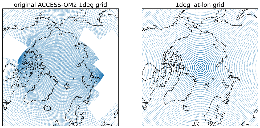
To regrid our fields we need to construct the three regridders for the three different resolutions using xesmf.Regridder(). The xesmf.Regridder() function takes as input two datasets, one that includes the original grid and one that includes the grids we need to regrid on. (Type ?xesmf.Regridder for the function’s docstring.)
The names of the coordinates need to follow CF-convetions. We also make sure to drop the 1D coords x and y to force the regridder to use the 2D arrays geolon_c and geolat_c.
Note: The 0.10 degree regridder_010degACCESSOM2_1deg below should take ~3-4 minutes to compute.
[10]:
%%time

regridder_1degACCESSOM2_1deg = xesmf.Regridder(
    ssh_1.drop_vars({"x", "y"}),
    ds_out,
    "bilinear",
    periodic=True,
    filename="bilinear_tracer_weights_in1degACCESSOM2_out1deg.nc",
)
regridder_1degACCESSOM2_1deg
CPU times: user 7.15 s, sys: 3.67 s, total: 10.8 s
Wall time: 12.5 s
[10]:
xESMF Regridder
Regridding algorithm:       bilinear
Weight filename:            bilinear_tracer_weights_in1degACCESSOM2_out1deg.nc
Reuse pre-computed weights? False
Input grid shape:           (300, 360)
Output grid shape:          (180, 360)
Periodic in longitude?      True
[11]:
%%time

regridder_025degACCESSOM2_1deg = xesmf.Regridder(
    ssh_025.drop_vars({"x", "y"}),
    ds_out,
    "bilinear",
    periodic=True,
    filename="bilinear_tracer_weights_in025degACCESSOM2_out1deg.nc",
)
regridder_025degACCESSOM2_1deg
CPU times: user 34.5 s, sys: 6.77 s, total: 41.2 s
Wall time: 26.6 s
[11]:
xESMF Regridder
Regridding algorithm:       bilinear
Weight filename:            bilinear_tracer_weights_in025degACCESSOM2_out1deg.nc
Reuse pre-computed weights? False
Input grid shape:           (1080, 1440)
Output grid shape:          (180, 360)
Periodic in longitude?      True
[12]:
%%time

regridder_010degACCESSOM2_1deg = xesmf.Regridder(
    ssh_010.drop_vars({"x", "y"}),
    ds_out,
    "bilinear",
    periodic=True,
    filename="bilinear_tracer_weights_in010degACCESSOM2_out1deg.nc",
)
regridder_010degACCESSOM2_1deg
CPU times: user 4min 3s, sys: 50.1 s, total: 4min 53s
Wall time: 3min 9s
[12]:
xESMF Regridder
Regridding algorithm:       bilinear
Weight filename:            bilinear_tracer_weights_in010degACCESSOM2_out1deg.nc
Reuse pre-computed weights? False
Input grid shape:           (2700, 3600)
Output grid shape:          (180, 360)
Periodic in longitude?      True
Note
For large grids (e.g., to regrid from a 0.10\(^\circ\) grid to a 0.20\(^\circ\)), it might take a while to compute the re-grid weights. But, once you compute the weights, you can construct a regridder using the already-computed weights from a netCDF file by providing with the reuse_weights = True argument, e.g.,
regridder = xesmf.Regridder(dataset_in, dataset_out, 'bilinear', periodic=True,
                            filename='weights_file.nc', reuse_weights=True)
or to automatically recalculate the weights file only in case it doesn’t already exist, do
import os

regridder = xesmf.Regridder(dataset_in, dataset_out, 'bilinear', periodic=True,
                            filename='weights_file.nc',
                            reuse_weights=os.path.exists('weights_file.nc'))
Let’s regrid our output
Now we use the regridders we constructed above to regrid our output. Note that the dimensions we are applying the re-gridding can’t be chunked, so when we opened the dataset, we set the chunks sizes to be the full size of x and y. The time axis can be chunked — for big datasets make sure that you rechunk time if needed so you don’t end up with huge chunk sizes. That is precisely why we used:
.chunk({'time': 'auto', 'longitude': -1, 'latitude': -1})
to ensure this.
Note also that for the regridded data arrays, we add back the longitude/latitude values on coords x/y respectively to make our lives easier with plotting later on.
[14]:
ssh_1_regridded = regridder_1degACCESSOM2_1deg(ssh_1)
ssh_1_regridded = ssh_1_regridded.drop_vars(["longitude", "latitude"])
ssh_1_regridded = ssh_1_regridded.assign_coords(
    {"x": ds_out.longitude.isel(y=0), "y": ds_out.latitude.isel(x=0)}
)
ssh_1_regridded = ssh_1_regridded.rename({"x": "longitude", "y": "latitude"})

ssh_1_regridded
[14]:
<xarray.DataArray (time: 24, latitude: 180, longitude: 360)> Size: 6MB
dask.array<astype, shape=(24, 180, 360), dtype=float32, chunksize=(24, 180, 360), chunktype=numpy.ndarray>
Coordinates:
  * time       (time) datetime64[ns] 192B 2000-01-14T12:00:00 ... 2001-12-14T...
  * latitude   (latitude) float64 1kB -89.5 -88.5 -87.5 -86.5 ... 87.5 88.5 89.5
  * longitude  (longitude) float64 3kB -279.5 -278.5 -277.5 ... 77.5 78.5 79.5
Attributes:
regrid_method: bilinear[15]:
ssh_025_regridded = regridder_025degACCESSOM2_1deg(ssh_025)
ssh_025_regridded = ssh_025_regridded.drop_vars(["longitude", "latitude"])
ssh_025_regridded = ssh_025_regridded.assign_coords(
    {"x": ds_out.longitude.isel(y=0), "y": ds_out.latitude.isel(x=0)}
)
ssh_025_regridded = ssh_025_regridded.rename({"x": "longitude", "y": "latitude"})
ssh_025_regridded
[15]:
<xarray.DataArray (time: 24, latitude: 180, longitude: 360)> Size: 6MB
dask.array<astype, shape=(24, 180, 360), dtype=float32, chunksize=(12, 180, 360), chunktype=numpy.ndarray>
Coordinates:
  * time       (time) datetime64[ns] 192B 2000-01-14T12:00:00 ... 2001-12-14T...
  * latitude   (latitude) float64 1kB -89.5 -88.5 -87.5 -86.5 ... 87.5 88.5 89.5
  * longitude  (longitude) float64 3kB -279.5 -278.5 -277.5 ... 77.5 78.5 79.5
Attributes:
regrid_method: bilinear[16]:
ssh_010_regridded = regridder_010degACCESSOM2_1deg(ssh_010)
ssh_010_regridded = ssh_010_regridded.drop_vars(["longitude", "latitude"])
ssh_010_regridded = ssh_010_regridded.assign_coords(
    {"x": ds_out.longitude.isel(y=0), "y": ds_out.latitude.isel(x=0)}
)
ssh_010_regridded = ssh_010_regridded.rename({"x": "longitude", "y": "latitude"})
ssh_010_regridded
[16]:
<xarray.DataArray (time: 24, latitude: 180, longitude: 360)> Size: 6MB
dask.array<astype, shape=(24, 180, 360), dtype=float32, chunksize=(3, 180, 360), chunktype=numpy.ndarray>
Coordinates:
  * time       (time) datetime64[ns] 192B 2000-01-16T12:00:00 ... 2001-12-16T...
  * latitude   (latitude) float64 1kB -89.5 -88.5 -87.5 -86.5 ... 87.5 88.5 89.5
  * longitude  (longitude) float64 3kB -279.5 -278.5 -277.5 ... 77.5 78.5 79.5
Attributes:
regrid_method: bilinearPlotting time
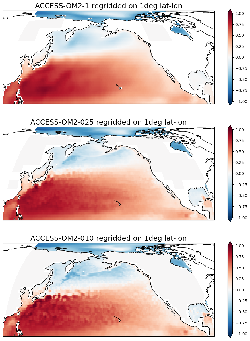
Now we can plot the regridded fields, slicing as we like using longitude and latitude coordinates. Here’s a comparisson of monthly-mean snapshots for sea-surface height in the North Pacific. Notice how things look “normal” north of 65\(^\circ\)N where the model’s grid has the tripolar complications!
[17]:
projection = ccrs.cartopy.crs.EqualEarth(central_longitude=180.0)

fig, axes = plt.subplots(
    nrows=3, subplot_kw={"projection": projection}, figsize=(12, 15)
)

for ax in axes:
    ax.coastlines()

ssh_1_regridded.isel(time=0).sel(
    {"longitude": slice(-250, -80), "latitude": slice(10, 90)}
).plot(
    ax=axes[0],
    transform=ccrs.PlateCarree(),
    extend="both",
    vmin=-1,
    vmax=1,
    cmap="RdBu_r",
)
axes[0].set_title("ACCESS-OM2-1 regridded on 1deg lat-lon", fontsize=18)

ssh_025_regridded.isel(time=0).sel(
    {"longitude": slice(-250, -80), "latitude": slice(10, 90)}
).plot(
    ax=axes[1],
    transform=ccrs.PlateCarree(),
    extend="both",
    vmin=-1,
    vmax=1,
    cmap="RdBu_r",
)

axes[1].set_title("ACCESS-OM2-025 regridded on 1deg lat-lon", fontsize=18)


ssh_010_regridded.isel(time=0).sel(
    {"longitude": slice(-250, -80), "latitude": slice(10, 90)}
).plot(
    ax=axes[2],
    transform=ccrs.PlateCarree(),
    extend="both",
    vmin=-1,
    vmax=1,
    cmap="RdBu_r",
)

axes[2].set_title("ACCESS-OM2-010 regridded on 1deg lat-lon", fontsize=18);
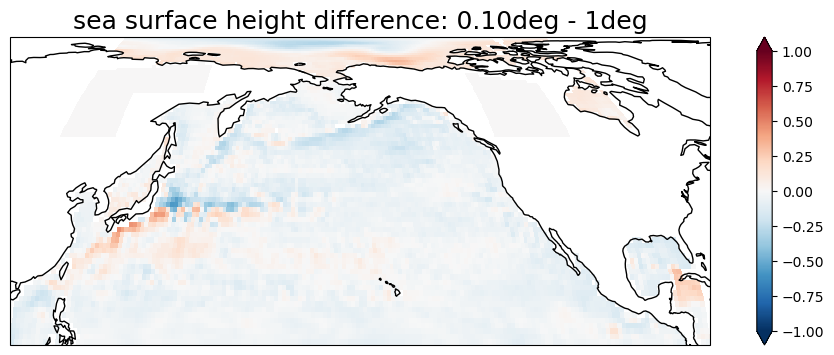
Another thing we can do now that we have everything on the same grid is to compute difference between fields from different model resolutions.
[18]:
plt.figure(figsize=(12, 4))
ax = plt.axes(projection=ccrs.cartopy.crs.EqualEarth(central_longitude=180.0))

(ssh_010_regridded.isel(time=0) - ssh_1_regridded.isel(time=0)).sel(
    {"longitude": slice(-250, -80), "latitude": slice(10, 90)}
).plot(
    ax=ax, transform=ccrs.PlateCarree(), extend="both", vmin=-1, vmax=1, cmap="RdBu_r"
)
ax.coastlines()
plt.title("sea surface height difference: 0.10deg - 1deg", fontsize=18);
/g/data/xp65/public/apps/med_conda/envs/analysis3-26.06/lib/python3.12/site-packages/distributed/client.py:3387: UserWarning: Sending large graph of size 12.71 MiB.
This may cause some slowdown.
Consider loading the data with Dask directly
 or using futures or delayed objects to embed the data into the graph without repetition.
See also https://docs.dask.org/en/stable/best-practices.html#load-data-with-dask for more information.
  warnings.warn(
Further examples
The example that compares sea ice observations with model outputs and also the “Regridders” section of the “Ice maps analysis” notebook include examples of functions that generate functions to regrid between ACCESS-OM2 resolutions and from various other datasets (JRA55, GIOMAS, and NSIDC) to the three ACCESS-OM2 resolutions. These regridder functions automatically save and reuse weights.
[18]:
client.close()