Extract variables at bottom of ocean: an example with Age
This notebook shows a simple example of plotting ocean Ideal Age. Ideal Age is a fictitious tracer which is set to zero in the surface grid-cell every timestep, and is aged by 1 year per year otherwise. It is a useful proxy for nutrients, such as carbon or oxygen (but not an exact analogue).
One of the interesting aspects of age is that we can use it to show pathways of the densest water in the ocean by plotting a map of age in the lowest grid cell. This plot requires a couple of tricks to extract information from the lowest cell.
Compute times were calculated using the (24 cpus, 95 Gb mem) Jupyter Lab on NCI’s Gadi with conda environment analysis3-25.07 or above.
st_ocean with the vertical coordinate of MOM6 data which is usually z_lht with the depth variable depthoagessc[1]:
import intake
import matplotlib.pyplot as plt
import xarray as xr
import numpy as np

import cartopy.crs as ccrs
import cmocean as cm

from dask.distributed import Client
[2]:
client = Client(threads_per_worker = 1)
client
[2]:
Client
Client-e6ad1c13-7511-11f1-a294-000003bdfe80
| Connection method: Cluster object | Cluster type: distributed.LocalCluster |
| Dashboard: /proxy/8787/status |
Cluster Info
LocalCluster
5a0599b0
| Dashboard: /proxy/8787/status | Workers: 28 |
| Total threads: 28 | Total memory: 251.19 GiB |
| Status: running | Using processes: True |
Scheduler Info
Scheduler
Scheduler-3ad343f3-2aba-40bc-85e5-65507b4a617b
| Comm: tcp://127.0.0.1:34231 | Workers: 0 |
| Dashboard: /proxy/8787/status | Total threads: 0 |
| Started: Just now | Total memory: 0 B |
Workers
Worker: 0
| Comm: tcp://127.0.0.1:34871 | Total threads: 1 |
| Dashboard: /proxy/46621/status | Memory: 8.97 GiB |
| Nanny: tcp://127.0.0.1:44085 | |
| Local directory: /jobfs/172784006.gadi-pbs/dask-scratch-space/worker-4_02xwk4 | |
Worker: 1
| Comm: tcp://127.0.0.1:43387 | Total threads: 1 |
| Dashboard: /proxy/44549/status | Memory: 8.97 GiB |
| Nanny: tcp://127.0.0.1:40149 | |
| Local directory: /jobfs/172784006.gadi-pbs/dask-scratch-space/worker-ml3_09s4 | |
Worker: 2
| Comm: tcp://127.0.0.1:38073 | Total threads: 1 |
| Dashboard: /proxy/39703/status | Memory: 8.97 GiB |
| Nanny: tcp://127.0.0.1:45119 | |
| Local directory: /jobfs/172784006.gadi-pbs/dask-scratch-space/worker-8_tgkp2j | |
Worker: 3
| Comm: tcp://127.0.0.1:36665 | Total threads: 1 |
| Dashboard: /proxy/38021/status | Memory: 8.97 GiB |
| Nanny: tcp://127.0.0.1:32963 | |
| Local directory: /jobfs/172784006.gadi-pbs/dask-scratch-space/worker-tx8ice3x | |
Worker: 4
| Comm: tcp://127.0.0.1:36597 | Total threads: 1 |
| Dashboard: /proxy/35755/status | Memory: 8.97 GiB |
| Nanny: tcp://127.0.0.1:33137 | |
| Local directory: /jobfs/172784006.gadi-pbs/dask-scratch-space/worker-jd4_1uo0 | |
Worker: 5
| Comm: tcp://127.0.0.1:37565 | Total threads: 1 |
| Dashboard: /proxy/43167/status | Memory: 8.97 GiB |
| Nanny: tcp://127.0.0.1:43651 | |
| Local directory: /jobfs/172784006.gadi-pbs/dask-scratch-space/worker-2usrt9g5 | |
Worker: 6
| Comm: tcp://127.0.0.1:38009 | Total threads: 1 |
| Dashboard: /proxy/38735/status | Memory: 8.97 GiB |
| Nanny: tcp://127.0.0.1:44541 | |
| Local directory: /jobfs/172784006.gadi-pbs/dask-scratch-space/worker-raegtds7 | |
Worker: 7
| Comm: tcp://127.0.0.1:41641 | Total threads: 1 |
| Dashboard: /proxy/36907/status | Memory: 8.97 GiB |
| Nanny: tcp://127.0.0.1:39993 | |
| Local directory: /jobfs/172784006.gadi-pbs/dask-scratch-space/worker-uf65y66f | |
Worker: 8
| Comm: tcp://127.0.0.1:33669 | Total threads: 1 |
| Dashboard: /proxy/38975/status | Memory: 8.97 GiB |
| Nanny: tcp://127.0.0.1:40753 | |
| Local directory: /jobfs/172784006.gadi-pbs/dask-scratch-space/worker-9bs2hlh4 | |
Worker: 9
| Comm: tcp://127.0.0.1:33847 | Total threads: 1 |
| Dashboard: /proxy/38787/status | Memory: 8.97 GiB |
| Nanny: tcp://127.0.0.1:33201 | |
| Local directory: /jobfs/172784006.gadi-pbs/dask-scratch-space/worker-6m7yer0c | |
Worker: 10
| Comm: tcp://127.0.0.1:44989 | Total threads: 1 |
| Dashboard: /proxy/46639/status | Memory: 8.97 GiB |
| Nanny: tcp://127.0.0.1:43787 | |
| Local directory: /jobfs/172784006.gadi-pbs/dask-scratch-space/worker-5sfhhdaj | |
Worker: 11
| Comm: tcp://127.0.0.1:34457 | Total threads: 1 |
| Dashboard: /proxy/39967/status | Memory: 8.97 GiB |
| Nanny: tcp://127.0.0.1:45275 | |
| Local directory: /jobfs/172784006.gadi-pbs/dask-scratch-space/worker-z1g7rwwz | |
Worker: 12
| Comm: tcp://127.0.0.1:46387 | Total threads: 1 |
| Dashboard: /proxy/32789/status | Memory: 8.97 GiB |
| Nanny: tcp://127.0.0.1:44141 | |
| Local directory: /jobfs/172784006.gadi-pbs/dask-scratch-space/worker-2gkd9s3y | |
Worker: 13
| Comm: tcp://127.0.0.1:44269 | Total threads: 1 |
| Dashboard: /proxy/34395/status | Memory: 8.97 GiB |
| Nanny: tcp://127.0.0.1:39733 | |
| Local directory: /jobfs/172784006.gadi-pbs/dask-scratch-space/worker-zm63_n4d | |
Worker: 14
| Comm: tcp://127.0.0.1:46365 | Total threads: 1 |
| Dashboard: /proxy/42999/status | Memory: 8.97 GiB |
| Nanny: tcp://127.0.0.1:38115 | |
| Local directory: /jobfs/172784006.gadi-pbs/dask-scratch-space/worker-4ou2fzz5 | |
Worker: 15
| Comm: tcp://127.0.0.1:41879 | Total threads: 1 |
| Dashboard: /proxy/40397/status | Memory: 8.97 GiB |
| Nanny: tcp://127.0.0.1:33255 | |
| Local directory: /jobfs/172784006.gadi-pbs/dask-scratch-space/worker-9v3wmx7t | |
Worker: 16
| Comm: tcp://127.0.0.1:35055 | Total threads: 1 |
| Dashboard: /proxy/43127/status | Memory: 8.97 GiB |
| Nanny: tcp://127.0.0.1:35241 | |
| Local directory: /jobfs/172784006.gadi-pbs/dask-scratch-space/worker-7_x66kvw | |
Worker: 17
| Comm: tcp://127.0.0.1:37215 | Total threads: 1 |
| Dashboard: /proxy/41061/status | Memory: 8.97 GiB |
| Nanny: tcp://127.0.0.1:44901 | |
| Local directory: /jobfs/172784006.gadi-pbs/dask-scratch-space/worker-qehqqe0m | |
Worker: 18
| Comm: tcp://127.0.0.1:40711 | Total threads: 1 |
| Dashboard: /proxy/42189/status | Memory: 8.97 GiB |
| Nanny: tcp://127.0.0.1:39557 | |
| Local directory: /jobfs/172784006.gadi-pbs/dask-scratch-space/worker-tadqagfz | |
Worker: 19
| Comm: tcp://127.0.0.1:43825 | Total threads: 1 |
| Dashboard: /proxy/45535/status | Memory: 8.97 GiB |
| Nanny: tcp://127.0.0.1:44963 | |
| Local directory: /jobfs/172784006.gadi-pbs/dask-scratch-space/worker-5zna1bl1 | |
Worker: 20
| Comm: tcp://127.0.0.1:45709 | Total threads: 1 |
| Dashboard: /proxy/46487/status | Memory: 8.97 GiB |
| Nanny: tcp://127.0.0.1:38251 | |
| Local directory: /jobfs/172784006.gadi-pbs/dask-scratch-space/worker-c945nc9e | |
Worker: 21
| Comm: tcp://127.0.0.1:40239 | Total threads: 1 |
| Dashboard: /proxy/38427/status | Memory: 8.97 GiB |
| Nanny: tcp://127.0.0.1:35999 | |
| Local directory: /jobfs/172784006.gadi-pbs/dask-scratch-space/worker-5cngcrgd | |
Worker: 22
| Comm: tcp://127.0.0.1:40433 | Total threads: 1 |
| Dashboard: /proxy/35779/status | Memory: 8.97 GiB |
| Nanny: tcp://127.0.0.1:34479 | |
| Local directory: /jobfs/172784006.gadi-pbs/dask-scratch-space/worker-x1qfyn4_ | |
Worker: 23
| Comm: tcp://127.0.0.1:41927 | Total threads: 1 |
| Dashboard: /proxy/38715/status | Memory: 8.97 GiB |
| Nanny: tcp://127.0.0.1:39459 | |
| Local directory: /jobfs/172784006.gadi-pbs/dask-scratch-space/worker-h6f8t_x9 | |
Worker: 24
| Comm: tcp://127.0.0.1:35199 | Total threads: 1 |
| Dashboard: /proxy/36273/status | Memory: 8.97 GiB |
| Nanny: tcp://127.0.0.1:39743 | |
| Local directory: /jobfs/172784006.gadi-pbs/dask-scratch-space/worker-ve68qtv4 | |
Worker: 25
| Comm: tcp://127.0.0.1:34551 | Total threads: 1 |
| Dashboard: /proxy/36003/status | Memory: 8.97 GiB |
| Nanny: tcp://127.0.0.1:40145 | |
| Local directory: /jobfs/172784006.gadi-pbs/dask-scratch-space/worker-dyx_op7b | |
Worker: 26
| Comm: tcp://127.0.0.1:38481 | Total threads: 1 |
| Dashboard: /proxy/33849/status | Memory: 8.97 GiB |
| Nanny: tcp://127.0.0.1:36667 | |
| Local directory: /jobfs/172784006.gadi-pbs/dask-scratch-space/worker-30b5krhg | |
Worker: 27
| Comm: tcp://127.0.0.1:46055 | Total threads: 1 |
| Dashboard: /proxy/46747/status | Memory: 8.97 GiB |
| Nanny: tcp://127.0.0.1:41533 | |
| Local directory: /jobfs/172784006.gadi-pbs/dask-scratch-space/worker-s8azlvdi | |
2026-07-01 16:00:21,038 - distributed.shuffle._scheduler_plugin - WARNING - Shuffle ef33bb80b017568def52fa9cadc8450e initialized by task ('rechunk-merge-rechunk-transfer-67a0106ae1c0a72625c1c3489af3d863', 0, 0, 3, 8, 0, 5, 3, 8) executed on worker tcp://127.0.0.1:41641
2026-07-01 16:00:21,139 - distributed.shuffle._scheduler_plugin - WARNING - Shuffle 36c706b679abb303c44342e2e4142718 initialized by task ('rechunk-merge-rechunk-transfer-67a0106ae1c0a72625c1c3489af3d863', 1, 0, 3, 7, 1, 5, 3, 7) executed on worker tcp://127.0.0.1:46055
2026-07-01 16:00:21,453 - distributed.shuffle._scheduler_plugin - WARNING - Shuffle 953c04d8a1cdb41634551a9fd8f04d57 initialized by task ('rechunk-merge-rechunk-transfer-67a0106ae1c0a72625c1c3489af3d863', 0, 0, 3, 7, 0, 5, 3, 7) executed on worker tcp://127.0.0.1:44989
2026-07-01 16:00:21,460 - distributed.shuffle._scheduler_plugin - WARNING - Shuffle aacd8f1e36e4cf4a9991bd2984682b57 initialized by task ('rechunk-merge-rechunk-transfer-67a0106ae1c0a72625c1c3489af3d863', 1, 0, 3, 8, 1, 5, 3, 8) executed on worker tcp://127.0.0.1:38481
2026-07-01 16:00:21,501 - distributed.shuffle._scheduler_plugin - WARNING - Shuffle 4b8a2462b55531d744369d4b396315f9 initialized by task ('rechunk-merge-rechunk-transfer-67a0106ae1c0a72625c1c3489af3d863', 0, 0, 3, 6, 0, 5, 3, 6) executed on worker tcp://127.0.0.1:44989
2026-07-01 16:00:21,559 - distributed.shuffle._scheduler_plugin - WARNING - Shuffle 28fc4e46b48dbeb35a72cc1343ac3a80 initialized by task ('rechunk-merge-rechunk-transfer-67a0106ae1c0a72625c1c3489af3d863', 1, 0, 3, 6, 1, 5, 3, 6) executed on worker tcp://127.0.0.1:41641
2026-07-01 16:00:22,075 - distributed.shuffle._scheduler_plugin - WARNING - Shuffle 95be3335d8272488a1569946ea03e24d initialized by task ('rechunk-merge-rechunk-transfer-67a0106ae1c0a72625c1c3489af3d863', 0, 0, 3, 4, 0, 5, 3, 4) executed on worker tcp://127.0.0.1:33669
2026-07-01 16:00:22,146 - distributed.shuffle._scheduler_plugin - WARNING - Shuffle 821636f2f826d9323ec1047cf7f9da8e initialized by task ('rechunk-merge-rechunk-transfer-67a0106ae1c0a72625c1c3489af3d863', 0, 0, 3, 5, 0, 5, 3, 5) executed on worker tcp://127.0.0.1:33669
2026-07-01 16:00:23,010 - distributed.shuffle._scheduler_plugin - WARNING - Shuffle e68a993c1868cf26f94a99a7c99cb989 initialized by task ('rechunk-merge-rechunk-transfer-67a0106ae1c0a72625c1c3489af3d863', 1, 0, 3, 5, 1, 3, 3, 5) executed on worker tcp://127.0.0.1:43825
2026-07-01 16:00:23,147 - distributed.shuffle._scheduler_plugin - WARNING - Shuffle 294d9ca3568c95bc2c9da8166014cb43 initialized by task ('rechunk-merge-rechunk-transfer-67a0106ae1c0a72625c1c3489af3d863', 1, 0, 3, 4, 1, 3, 3, 4) executed on worker tcp://127.0.0.1:43825
2026-07-01 16:00:23,324 - distributed.shuffle._scheduler_plugin - WARNING - Shuffle 2b2f6ff052b449424b0d4def81044ecc initialized by task ('rechunk-merge-rechunk-transfer-67a0106ae1c0a72625c1c3489af3d863', 0, 0, 3, 3, 0, 5, 3, 3) executed on worker tcp://127.0.0.1:46365
2026-07-01 16:00:23,349 - distributed.shuffle._scheduler_plugin - WARNING - Shuffle ef33bb80b017568def52fa9cadc8450e deactivated due to stimulus 'task-finished-1782885623.325747'
2026-07-01 16:00:23,377 - distributed.shuffle._scheduler_plugin - WARNING - Shuffle 6709ec766a065ed47f675df7c5bb17cb initialized by task ('rechunk-merge-rechunk-transfer-67a0106ae1c0a72625c1c3489af3d863', 0, 0, 3, 2, 0, 5, 3, 2) executed on worker tcp://127.0.0.1:46365
2026-07-01 16:00:23,488 - distributed.shuffle._scheduler_plugin - WARNING - Shuffle 953c04d8a1cdb41634551a9fd8f04d57 deactivated due to stimulus 'task-finished-1782885623.4384215'
2026-07-01 16:00:23,892 - distributed.shuffle._scheduler_plugin - WARNING - Shuffle 4b8a2462b55531d744369d4b396315f9 deactivated due to stimulus 'task-finished-1782885623.868836'
2026-07-01 16:00:23,936 - distributed.shuffle._scheduler_plugin - WARNING - Shuffle 5cea2f05684c6f95fcfec530685881f3 initialized by task ('rechunk-merge-rechunk-transfer-67a0106ae1c0a72625c1c3489af3d863', 1, 0, 3, 3, 1, 5, 3, 3) executed on worker tcp://127.0.0.1:40711
2026-07-01 16:00:24,154 - distributed.shuffle._scheduler_plugin - WARNING - Shuffle ca285a4f5c0890ba023bb2615b1451c4 initialized by task ('rechunk-merge-rechunk-transfer-67a0106ae1c0a72625c1c3489af3d863', 1, 0, 3, 2, 1, 5, 3, 2) executed on worker tcp://127.0.0.1:40711
2026-07-01 16:00:24,235 - distributed.shuffle._scheduler_plugin - WARNING - Shuffle 36c706b679abb303c44342e2e4142718 deactivated due to stimulus 'task-finished-1782885624.206823'
2026-07-01 16:00:24,425 - distributed.shuffle._scheduler_plugin - WARNING - Shuffle e846804a18e2d55b4e815999bd449f5f initialized by task ('rechunk-merge-rechunk-transfer-67a0106ae1c0a72625c1c3489af3d863', 0, 0, 3, 1, 0, 5, 3, 1) executed on worker tcp://127.0.0.1:38009
2026-07-01 16:00:24,540 - distributed.shuffle._scheduler_plugin - WARNING - Shuffle 6cfad5cc8c307f50e1a93ba3cd832c81 initialized by task ('rechunk-merge-rechunk-transfer-67a0106ae1c0a72625c1c3489af3d863', 0, 0, 3, 0, 0, 5, 3, 0) executed on worker tcp://127.0.0.1:38009
2026-07-01 16:00:24,640 - distributed.shuffle._scheduler_plugin - WARNING - Shuffle aacd8f1e36e4cf4a9991bd2984682b57 deactivated due to stimulus 'task-finished-1782885624.6325552'
2026-07-01 16:00:24,899 - distributed.shuffle._scheduler_plugin - WARNING - Shuffle 821636f2f826d9323ec1047cf7f9da8e deactivated due to stimulus 'task-finished-1782885624.844865'
2026-07-01 16:00:25,039 - distributed.shuffle._scheduler_plugin - WARNING - Shuffle 28fc4e46b48dbeb35a72cc1343ac3a80 deactivated due to stimulus 'task-finished-1782885625.0253708'
2026-07-01 16:00:25,232 - distributed.shuffle._scheduler_plugin - WARNING - Shuffle 95be3335d8272488a1569946ea03e24d deactivated due to stimulus 'task-finished-1782885625.2173576'
2026-07-01 16:00:25,292 - distributed.shuffle._scheduler_plugin - WARNING - Shuffle f48e8ee6db13a7efc5a26dbe4e17ad35 initialized by task ('rechunk-merge-rechunk-transfer-67a0106ae1c0a72625c1c3489af3d863', 1, 0, 3, 1, 1, 5, 3, 1) executed on worker tcp://127.0.0.1:46365
2026-07-01 16:00:25,323 - distributed.shuffle._scheduler_plugin - WARNING - Shuffle b3e482fd6b60b78587f66494ecbb1d23 initialized by task ('rechunk-merge-rechunk-transfer-67a0106ae1c0a72625c1c3489af3d863', 1, 0, 3, 0, 1, 4, 3, 0) executed on worker tcp://127.0.0.1:34457
2026-07-01 16:00:25,325 - distributed.shuffle._scheduler_plugin - WARNING - Shuffle e68a993c1868cf26f94a99a7c99cb989 deactivated due to stimulus 'task-finished-1782885625.2952585'
2026-07-01 16:00:25,614 - distributed.shuffle._scheduler_plugin - WARNING - Shuffle 6709ec766a065ed47f675df7c5bb17cb deactivated due to stimulus 'task-finished-1782885625.6036413'
2026-07-01 16:00:25,828 - distributed.shuffle._scheduler_plugin - WARNING - Shuffle 5f6718f2fb725063fb9846feb037fb2e initialized by task ('rechunk-merge-rechunk-transfer-67a0106ae1c0a72625c1c3489af3d863', 0, 0, 2, 6, 0, 5, 2, 6) executed on worker tcp://127.0.0.1:38481
2026-07-01 16:00:25,978 - distributed.shuffle._scheduler_plugin - WARNING - Shuffle 294d9ca3568c95bc2c9da8166014cb43 deactivated due to stimulus 'task-finished-1782885625.9754798'
2026-07-01 16:00:26,042 - distributed.shuffle._scheduler_plugin - WARNING - Shuffle 2b2f6ff052b449424b0d4def81044ecc deactivated due to stimulus 'task-finished-1782885626.005743'
2026-07-01 16:00:26,106 - distributed.shuffle._scheduler_plugin - WARNING - Shuffle e846804a18e2d55b4e815999bd449f5f deactivated due to stimulus 'task-finished-1782885626.0844765'
2026-07-01 16:00:26,178 - distributed.shuffle._scheduler_plugin - WARNING - Shuffle 305dbb0c2c5472108153e193b73929bb initialized by task ('rechunk-merge-rechunk-transfer-67a0106ae1c0a72625c1c3489af3d863', 0, 0, 2, 8, 0, 3, 2, 8) executed on worker tcp://127.0.0.1:38481
2026-07-01 16:00:26,232 - distributed.shuffle._scheduler_plugin - WARNING - Shuffle 1a766d5654e36ba571412de932e49a36 initialized by task ('rechunk-merge-rechunk-transfer-67a0106ae1c0a72625c1c3489af3d863', 0, 0, 2, 7, 0, 5, 2, 7) executed on worker tcp://127.0.0.1:37565
2026-07-01 16:00:26,331 - distributed.shuffle._scheduler_plugin - WARNING - Shuffle ca285a4f5c0890ba023bb2615b1451c4 deactivated due to stimulus 'task-finished-1782885626.302742'
2026-07-01 16:00:26,508 - distributed.shuffle._scheduler_plugin - WARNING - Shuffle 461d0dd73783293effdf3cdd6d51aba4 initialized by task ('rechunk-merge-rechunk-transfer-67a0106ae1c0a72625c1c3489af3d863', 1, 0, 2, 6, 1, 5, 2, 6) executed on worker tcp://127.0.0.1:34457
2026-07-01 16:00:26,572 - distributed.shuffle._scheduler_plugin - WARNING - Shuffle dc6ea520d88479a7ddca7460d7fd2aa5 initialized by task ('rechunk-merge-rechunk-transfer-67a0106ae1c0a72625c1c3489af3d863', 1, 0, 2, 8, 1, 5, 2, 8) executed on worker tcp://127.0.0.1:41641
2026-07-01 16:00:26,583 - distributed.shuffle._scheduler_plugin - WARNING - Shuffle d99cbe2070489a83b760cd7470daf0e9 initialized by task ('rechunk-merge-rechunk-transfer-67a0106ae1c0a72625c1c3489af3d863', 1, 0, 2, 7, 1, 5, 2, 7) executed on worker tcp://127.0.0.1:46055
2026-07-01 16:00:26,630 - distributed.shuffle._scheduler_plugin - WARNING - Shuffle 5cea2f05684c6f95fcfec530685881f3 deactivated due to stimulus 'task-finished-1782885626.604152'
2026-07-01 16:00:27,099 - distributed.shuffle._scheduler_plugin - WARNING - Shuffle 6cfad5cc8c307f50e1a93ba3cd832c81 deactivated due to stimulus 'task-finished-1782885627.0820243'
2026-07-01 16:00:27,469 - distributed.shuffle._scheduler_plugin - WARNING - Shuffle f48e8ee6db13a7efc5a26dbe4e17ad35 deactivated due to stimulus 'task-finished-1782885627.462813'
2026-07-01 16:00:27,975 - distributed.shuffle._scheduler_plugin - WARNING - Shuffle b3e482fd6b60b78587f66494ecbb1d23 deactivated due to stimulus 'task-finished-1782885627.9634845'
2026-07-01 16:00:28,059 - distributed.shuffle._scheduler_plugin - WARNING - Shuffle 305dbb0c2c5472108153e193b73929bb deactivated due to stimulus 'task-finished-1782885628.0311298'
2026-07-01 16:00:28,112 - distributed.shuffle._scheduler_plugin - WARNING - Shuffle 81fd7c2adc0d548b253ec4c3ab72056f initialized by task ('rechunk-merge-rechunk-transfer-67a0106ae1c0a72625c1c3489af3d863', 0, 0, 2, 5, 0, 5, 2, 5) executed on worker tcp://127.0.0.1:35055
2026-07-01 16:00:28,190 - distributed.shuffle._scheduler_plugin - WARNING - Shuffle f518485413417a0e48e3ae298b5f5cf3 initialized by task ('rechunk-merge-rechunk-transfer-67a0106ae1c0a72625c1c3489af3d863', 0, 0, 2, 4, 0, 5, 2, 4) executed on worker tcp://127.0.0.1:35055
2026-07-01 16:00:28,320 - distributed.shuffle._scheduler_plugin - WARNING - Shuffle 8ab20898c1ebaf3172ad8febf2b712c0 initialized by task ('rechunk-merge-rechunk-transfer-67a0106ae1c0a72625c1c3489af3d863', 1, 0, 2, 4, 1, 5, 2, 4) executed on worker tcp://127.0.0.1:37215
2026-07-01 16:00:28,364 - distributed.shuffle._scheduler_plugin - WARNING - Shuffle 2a5a9f5d0bd0a60b0fe57bbe644b9bee initialized by task ('rechunk-merge-rechunk-transfer-67a0106ae1c0a72625c1c3489af3d863', 1, 0, 2, 5, 1, 5, 2, 5) executed on worker tcp://127.0.0.1:34457
2026-07-01 16:00:28,541 - distributed.shuffle._scheduler_plugin - WARNING - Shuffle 1a766d5654e36ba571412de932e49a36 deactivated due to stimulus 'task-finished-1782885628.5314622'
2026-07-01 16:00:28,810 - distributed.shuffle._scheduler_plugin - WARNING - Shuffle 5f6718f2fb725063fb9846feb037fb2e deactivated due to stimulus 'task-finished-1782885628.7771761'
2026-07-01 16:00:29,133 - distributed.shuffle._scheduler_plugin - WARNING - Shuffle dc6ea520d88479a7ddca7460d7fd2aa5 deactivated due to stimulus 'task-finished-1782885629.1245189'
2026-07-01 16:00:29,140 - distributed.shuffle._scheduler_plugin - WARNING - Shuffle 854d04b5cfc2cff2b9acbc83292bc8bd initialized by task ('rechunk-merge-rechunk-transfer-67a0106ae1c0a72625c1c3489af3d863', 0, 0, 2, 3, 0, 4, 2, 3) executed on worker tcp://127.0.0.1:41641
2026-07-01 16:00:29,219 - distributed.shuffle._scheduler_plugin - WARNING - Shuffle 78dabc4ab8ae9bb2770998987fede8e6 initialized by task ('rechunk-merge-rechunk-transfer-67a0106ae1c0a72625c1c3489af3d863', 0, 0, 2, 2, 0, 4, 2, 2) executed on worker tcp://127.0.0.1:41641
2026-07-01 16:00:29,318 - distributed.shuffle._scheduler_plugin - WARNING - Shuffle e59c1a3ae4fd025fa37bfbff5e72a252 initialized by task ('rechunk-merge-rechunk-transfer-67a0106ae1c0a72625c1c3489af3d863', 1, 0, 2, 3, 1, 5, 2, 3) executed on worker tcp://127.0.0.1:46055
2026-07-01 16:00:29,706 - distributed.shuffle._scheduler_plugin - WARNING - Shuffle 267921aec10458fbf314522aa9efeeb0 initialized by task ('rechunk-merge-rechunk-transfer-67a0106ae1c0a72625c1c3489af3d863', 1, 0, 2, 2, 1, 5, 2, 2) executed on worker tcp://127.0.0.1:40433
2026-07-01 16:00:30,054 - distributed.shuffle._scheduler_plugin - WARNING - Shuffle d99cbe2070489a83b760cd7470daf0e9 deactivated due to stimulus 'task-finished-1782885630.0286763'
2026-07-01 16:00:30,093 - distributed.shuffle._scheduler_plugin - WARNING - Shuffle 461d0dd73783293effdf3cdd6d51aba4 deactivated due to stimulus 'task-finished-1782885630.0869944'
2026-07-01 16:00:30,532 - distributed.shuffle._scheduler_plugin - WARNING - Shuffle b29e4d46a08b24b50887a75dcec7144a initialized by task ('rechunk-merge-rechunk-transfer-67a0106ae1c0a72625c1c3489af3d863', 1, 0, 2, 1, 1, 5, 2, 1) executed on worker tcp://127.0.0.1:41641
2026-07-01 16:00:30,568 - distributed.shuffle._scheduler_plugin - WARNING - Shuffle f518485413417a0e48e3ae298b5f5cf3 deactivated due to stimulus 'task-finished-1782885630.528421'
2026-07-01 16:00:30,577 - distributed.shuffle._scheduler_plugin - WARNING - Shuffle 7b02894e10946b4523d365a470741913 initialized by task ('rechunk-merge-rechunk-transfer-67a0106ae1c0a72625c1c3489af3d863', 0, 0, 2, 1, 0, 5, 2, 1) executed on worker tcp://127.0.0.1:36597
2026-07-01 16:00:30,637 - distributed.shuffle._scheduler_plugin - WARNING - Shuffle e7d2024118b3fa41ffcf0b8641620c50 initialized by task ('rechunk-merge-rechunk-transfer-67a0106ae1c0a72625c1c3489af3d863', 1, 0, 2, 0, 1, 5, 2, 0) executed on worker tcp://127.0.0.1:41641
2026-07-01 16:00:30,656 - distributed.shuffle._scheduler_plugin - WARNING - Shuffle 81fd7c2adc0d548b253ec4c3ab72056f deactivated due to stimulus 'task-finished-1782885630.627924'
2026-07-01 16:00:30,677 - distributed.shuffle._scheduler_plugin - WARNING - Shuffle 7b6f14a74648dabeb7d59f8ce88254da initialized by task ('rechunk-merge-rechunk-transfer-67a0106ae1c0a72625c1c3489af3d863', 0, 0, 2, 0, 0, 5, 2, 0) executed on worker tcp://127.0.0.1:41879
2026-07-01 16:00:31,020 - distributed.shuffle._scheduler_plugin - WARNING - Shuffle 2a5a9f5d0bd0a60b0fe57bbe644b9bee deactivated due to stimulus 'task-finished-1782885631.0137239'
2026-07-01 16:00:31,177 - distributed.shuffle._scheduler_plugin - WARNING - Shuffle 8b2dca9e61ad06764de0cb779833f3dd initialized by task ('rechunk-merge-rechunk-transfer-67a0106ae1c0a72625c1c3489af3d863', 0, 0, 1, 6, 0, 5, 1, 6) executed on worker tcp://127.0.0.1:40711
2026-07-01 16:00:31,202 - distributed.shuffle._scheduler_plugin - WARNING - Shuffle 78dabc4ab8ae9bb2770998987fede8e6 deactivated due to stimulus 'task-finished-1782885631.198993'
2026-07-01 16:00:31,416 - distributed.shuffle._scheduler_plugin - WARNING - Shuffle 8ab20898c1ebaf3172ad8febf2b712c0 deactivated due to stimulus 'task-finished-1782885631.4049656'
2026-07-01 16:00:31,423 - distributed.shuffle._scheduler_plugin - WARNING - Shuffle b756aef7655f9c1a949cba122ec91530 initialized by task ('rechunk-merge-rechunk-transfer-67a0106ae1c0a72625c1c3489af3d863', 0, 0, 1, 8, 0, 5, 1, 8) executed on worker tcp://127.0.0.1:35055
2026-07-01 16:00:31,748 - distributed.shuffle._scheduler_plugin - WARNING - Shuffle 854d04b5cfc2cff2b9acbc83292bc8bd deactivated due to stimulus 'task-finished-1782885631.7374008'
2026-07-01 16:00:31,816 - distributed.shuffle._scheduler_plugin - WARNING - Shuffle 507995dcff3929e42d04ff22b7171bac initialized by task ('rechunk-merge-rechunk-transfer-67a0106ae1c0a72625c1c3489af3d863', 0, 0, 1, 7, 0, 5, 1, 7) executed on worker tcp://127.0.0.1:40711
2026-07-01 16:00:31,874 - distributed.shuffle._scheduler_plugin - WARNING - Shuffle 5c090f01aed4781ead692d87d9b4ea6a initialized by task ('rechunk-merge-rechunk-transfer-67a0106ae1c0a72625c1c3489af3d863', 1, 0, 1, 8, 1, 5, 1, 8) executed on worker tcp://127.0.0.1:35199
2026-07-01 16:00:31,956 - distributed.shuffle._scheduler_plugin - WARNING - Shuffle e59c1a3ae4fd025fa37bfbff5e72a252 deactivated due to stimulus 'task-finished-1782885631.9316425'
2026-07-01 16:00:32,056 - distributed.shuffle._scheduler_plugin - WARNING - Shuffle 7b02894e10946b4523d365a470741913 deactivated due to stimulus 'task-finished-1782885632.0361092'
2026-07-01 16:00:32,225 - distributed.shuffle._scheduler_plugin - WARNING - Shuffle 7b6f14a74648dabeb7d59f8ce88254da deactivated due to stimulus 'task-finished-1782885632.2082577'
2026-07-01 16:00:32,301 - distributed.shuffle._scheduler_plugin - WARNING - Shuffle 267921aec10458fbf314522aa9efeeb0 deactivated due to stimulus 'task-finished-1782885632.2915661'
2026-07-01 16:00:32,908 - distributed.shuffle._scheduler_plugin - WARNING - Shuffle 50131514730f16620da7b82479bab574 initialized by task ('rechunk-merge-rechunk-transfer-67a0106ae1c0a72625c1c3489af3d863', 1, 0, 1, 6, 1, 5, 1, 6) executed on worker tcp://127.0.0.1:37565
2026-07-01 16:00:32,980 - distributed.shuffle._scheduler_plugin - WARNING - Shuffle 839def652036851f1bb01af81242955b initialized by task ('rechunk-merge-rechunk-transfer-67a0106ae1c0a72625c1c3489af3d863', 0, 0, 1, 4, 0, 5, 1, 4) executed on worker tcp://127.0.0.1:40239
2026-07-01 16:00:33,044 - distributed.shuffle._scheduler_plugin - WARNING - Shuffle b2a24c28963e17bf3b08ec59f3db922c initialized by task ('rechunk-merge-rechunk-transfer-67a0106ae1c0a72625c1c3489af3d863', 0, 0, 1, 5, 0, 5, 1, 5) executed on worker tcp://127.0.0.1:34457
2026-07-01 16:00:33,052 - distributed.shuffle._scheduler_plugin - WARNING - Shuffle a755e86a47e3dff2707aedee0d9fcc47 initialized by task ('rechunk-merge-rechunk-transfer-67a0106ae1c0a72625c1c3489af3d863', 1, 0, 1, 7, 1, 5, 1, 7) executed on worker tcp://127.0.0.1:37565
2026-07-01 16:00:33,354 - distributed.shuffle._scheduler_plugin - WARNING - Shuffle b29e4d46a08b24b50887a75dcec7144a deactivated due to stimulus 'task-finished-1782885633.3393874'
2026-07-01 16:00:33,415 - distributed.shuffle._scheduler_plugin - WARNING - Shuffle cda1e72d2c972876386a5cb1b6e231b4 initialized by task ('rechunk-merge-rechunk-transfer-67a0106ae1c0a72625c1c3489af3d863', 1, 0, 1, 5, 1, 5, 1, 5) executed on worker tcp://127.0.0.1:34551
2026-07-01 16:00:33,505 - distributed.shuffle._scheduler_plugin - WARNING - Shuffle e7d2024118b3fa41ffcf0b8641620c50 deactivated due to stimulus 'task-finished-1782885633.4994512'
2026-07-01 16:00:33,650 - distributed.shuffle._scheduler_plugin - WARNING - Shuffle b756aef7655f9c1a949cba122ec91530 deactivated due to stimulus 'task-finished-1782885633.6362145'
2026-07-01 16:00:33,724 - distributed.shuffle._scheduler_plugin - WARNING - Shuffle aaf36c9e65d823b00c35a31257246e03 initialized by task ('rechunk-merge-rechunk-transfer-67a0106ae1c0a72625c1c3489af3d863', 1, 0, 1, 4, 1, 5, 1, 4) executed on worker tcp://127.0.0.1:43387
2026-07-01 16:00:33,783 - distributed.shuffle._scheduler_plugin - WARNING - Shuffle 8b2dca9e61ad06764de0cb779833f3dd deactivated due to stimulus 'task-finished-1782885633.769035'
2026-07-01 16:00:34,818 - distributed.shuffle._scheduler_plugin - WARNING - Shuffle 119ea8f3f78ad0519e439b7c8cbb7d3c initialized by task ('rechunk-merge-rechunk-transfer-67a0106ae1c0a72625c1c3489af3d863', 0, 0, 1, 3, 0, 5, 1, 3) executed on worker tcp://127.0.0.1:38073
2026-07-01 16:00:34,876 - distributed.shuffle._scheduler_plugin - WARNING - Shuffle b30f15acbda00750f8c071578ffde1ba initialized by task ('rechunk-merge-rechunk-transfer-67a0106ae1c0a72625c1c3489af3d863', 0, 0, 1, 2, 0, 5, 1, 2) executed on worker tcp://127.0.0.1:38073
2026-07-01 16:00:34,975 - distributed.shuffle._scheduler_plugin - WARNING - Shuffle 507995dcff3929e42d04ff22b7171bac deactivated due to stimulus 'task-finished-1782885634.9610093'
2026-07-01 16:00:35,092 - distributed.shuffle._scheduler_plugin - WARNING - Shuffle ac7bed35874dc1ca56db005d99133eba initialized by task ('rechunk-merge-rechunk-transfer-67a0106ae1c0a72625c1c3489af3d863', 1, 0, 1, 3, 1, 5, 1, 3) executed on worker tcp://127.0.0.1:37565
2026-07-01 16:00:35,094 - distributed.shuffle._scheduler_plugin - WARNING - Shuffle e9fc2f368984eb6531e365794bfded46 initialized by task ('rechunk-merge-rechunk-transfer-67a0106ae1c0a72625c1c3489af3d863', 1, 0, 1, 2, 1, 5, 1, 2) executed on worker tcp://127.0.0.1:33847
2026-07-01 16:00:35,396 - distributed.shuffle._scheduler_plugin - WARNING - Shuffle 5c090f01aed4781ead692d87d9b4ea6a deactivated due to stimulus 'task-finished-1782885635.3738167'
2026-07-01 16:00:35,640 - distributed.shuffle._scheduler_plugin - WARNING - Shuffle dd4050f36ad128243a1b9c14eeb1f440 initialized by task ('rechunk-merge-rechunk-transfer-67a0106ae1c0a72625c1c3489af3d863', 0, 0, 1, 1, 0, 5, 1, 1) executed on worker tcp://127.0.0.1:34871
2026-07-01 16:00:35,819 - distributed.shuffle._scheduler_plugin - WARNING - Shuffle 0505a448c772ba991a15b2abca095d22 initialized by task ('rechunk-merge-rechunk-transfer-67a0106ae1c0a72625c1c3489af3d863', 0, 0, 1, 0, 0, 4, 1, 0) executed on worker tcp://127.0.0.1:44989
2026-07-01 16:00:36,064 - distributed.shuffle._scheduler_plugin - WARNING - Shuffle 839def652036851f1bb01af81242955b deactivated due to stimulus 'task-finished-1782885636.036603'
2026-07-01 16:00:36,130 - distributed.shuffle._scheduler_plugin - WARNING - Shuffle b2a24c28963e17bf3b08ec59f3db922c deactivated due to stimulus 'task-finished-1782885636.113459'
2026-07-01 16:00:36,164 - distributed.shuffle._scheduler_plugin - WARNING - Shuffle 50131514730f16620da7b82479bab574 deactivated due to stimulus 'task-finished-1782885636.1437018'
2026-07-01 16:00:36,191 - distributed.shuffle._scheduler_plugin - WARNING - Shuffle 9b4e6be9bb71274ae62d004868762a78 initialized by task ('rechunk-merge-rechunk-transfer-67a0106ae1c0a72625c1c3489af3d863', 1, 0, 1, 1, 1, 5, 1, 1) executed on worker tcp://127.0.0.1:37565
2026-07-01 16:00:36,238 - distributed.shuffle._scheduler_plugin - WARNING - Shuffle 8bd61b53991ef8c43cbb1b58bbb2e610 initialized by task ('rechunk-merge-rechunk-transfer-67a0106ae1c0a72625c1c3489af3d863', 1, 0, 1, 0, 1, 5, 1, 0) executed on worker tcp://127.0.0.1:33669
2026-07-01 16:00:36,449 - distributed.shuffle._scheduler_plugin - WARNING - Shuffle cda1e72d2c972876386a5cb1b6e231b4 deactivated due to stimulus 'task-finished-1782885636.4302468'
2026-07-01 16:00:36,500 - distributed.shuffle._scheduler_plugin - WARNING - Shuffle a755e86a47e3dff2707aedee0d9fcc47 deactivated due to stimulus 'task-finished-1782885636.4851115'
2026-07-01 16:00:36,790 - distributed.shuffle._scheduler_plugin - WARNING - Shuffle a14b82bd004fdfda87e30ccb83409e87 initialized by task ('rechunk-merge-rechunk-transfer-67a0106ae1c0a72625c1c3489af3d863', 0, 0, 0, 6, 0, 5, 0, 6) executed on worker tcp://127.0.0.1:34871
2026-07-01 16:00:36,792 - distributed.shuffle._scheduler_plugin - WARNING - Shuffle 1ff241c0bfd4c3f199fa64313efc023c initialized by task ('rechunk-merge-rechunk-transfer-67a0106ae1c0a72625c1c3489af3d863', 0, 0, 0, 8, 0, 5, 0, 8) executed on worker tcp://127.0.0.1:46055
2026-07-01 16:00:36,811 - distributed.shuffle._scheduler_plugin - WARNING - Shuffle aaf36c9e65d823b00c35a31257246e03 deactivated due to stimulus 'task-finished-1782885636.7879384'
2026-07-01 16:00:36,853 - distributed.shuffle._scheduler_plugin - WARNING - Shuffle 482c01b8b6aaa5dfe439d0ae20a204ae initialized by task ('rechunk-merge-rechunk-transfer-67a0106ae1c0a72625c1c3489af3d863', 0, 0, 0, 7, 0, 5, 0, 7) executed on worker tcp://127.0.0.1:34871
2026-07-01 16:00:36,933 - distributed.shuffle._scheduler_plugin - WARNING - Shuffle ac7bed35874dc1ca56db005d99133eba deactivated due to stimulus 'task-finished-1782885636.9112966'
2026-07-01 16:00:37,066 - distributed.shuffle._scheduler_plugin - WARNING - Shuffle 119ea8f3f78ad0519e439b7c8cbb7d3c deactivated due to stimulus 'task-finished-1782885637.0449543'
2026-07-01 16:00:37,435 - distributed.shuffle._scheduler_plugin - WARNING - Shuffle e9fc2f368984eb6531e365794bfded46 deactivated due to stimulus 'task-finished-1782885637.418329'
2026-07-01 16:00:37,658 - distributed.shuffle._scheduler_plugin - WARNING - Shuffle cc675be92a62cc023aab9607e94ec77f initialized by task ('rechunk-merge-rechunk-transfer-67a0106ae1c0a72625c1c3489af3d863', 1, 0, 0, 6, 1, 5, 0, 6) executed on worker tcp://127.0.0.1:44269
2026-07-01 16:00:37,751 - distributed.shuffle._scheduler_plugin - WARNING - Shuffle b30f15acbda00750f8c071578ffde1ba deactivated due to stimulus 'task-finished-1782885637.7363725'
2026-07-01 16:00:37,872 - distributed.shuffle._scheduler_plugin - WARNING - Shuffle d7fcabcf055c13989775a6339f2ad006 initialized by task ('rechunk-merge-rechunk-transfer-67a0106ae1c0a72625c1c3489af3d863', 1, 0, 0, 7, 1, 5, 0, 7) executed on worker tcp://127.0.0.1:46387
2026-07-01 16:00:37,880 - distributed.shuffle._scheduler_plugin - WARNING - Shuffle b2021187a33e49db22bec2f5e4469729 initialized by task ('rechunk-merge-rechunk-transfer-67a0106ae1c0a72625c1c3489af3d863', 1, 0, 0, 8, 1, 4, 0, 8) executed on worker tcp://127.0.0.1:37565
2026-07-01 16:00:38,493 - distributed.shuffle._scheduler_plugin - WARNING - Shuffle 9b4e6be9bb71274ae62d004868762a78 deactivated due to stimulus 'task-finished-1782885638.0173857'
2026-07-01 16:00:38,566 - distributed.shuffle._scheduler_plugin - WARNING - Shuffle dd4050f36ad128243a1b9c14eeb1f440 deactivated due to stimulus 'task-finished-1782885638.4283383'
2026-07-01 16:00:39,151 - distributed.shuffle._scheduler_plugin - WARNING - Shuffle d092807acab9046425c25a3939fa7a79 initialized by task ('rechunk-merge-rechunk-transfer-67a0106ae1c0a72625c1c3489af3d863', 0, 0, 0, 4, 0, 4, 0, 4) executed on worker tcp://127.0.0.1:43387
2026-07-01 16:00:39,160 - distributed.shuffle._scheduler_plugin - WARNING - Shuffle 8bd61b53991ef8c43cbb1b58bbb2e610 deactivated due to stimulus 'task-finished-1782885639.153208'
2026-07-01 16:00:39,172 - distributed.shuffle._scheduler_plugin - WARNING - Shuffle 26fdbeae2f916e534af7949b8c73d9b4 initialized by task ('rechunk-merge-rechunk-transfer-67a0106ae1c0a72625c1c3489af3d863', 0, 0, 0, 5, 0, 4, 0, 5) executed on worker tcp://127.0.0.1:35199
2026-07-01 16:00:39,621 - distributed.shuffle._scheduler_plugin - WARNING - Shuffle 0505a448c772ba991a15b2abca095d22 deactivated due to stimulus 'task-finished-1782885639.6178725'
2026-07-01 16:00:39,758 - distributed.shuffle._scheduler_plugin - WARNING - Shuffle 549e66d9340684eae37886b932f07960 initialized by task ('rechunk-merge-rechunk-transfer-67a0106ae1c0a72625c1c3489af3d863', 1, 0, 0, 4, 1, 5, 0, 4) executed on worker tcp://127.0.0.1:43825
2026-07-01 16:00:39,856 - distributed.shuffle._scheduler_plugin - WARNING - Shuffle 180a255983365d6e6099822d9ed308f0 initialized by task ('rechunk-merge-rechunk-transfer-67a0106ae1c0a72625c1c3489af3d863', 1, 0, 0, 5, 1, 5, 0, 5) executed on worker tcp://127.0.0.1:34871
2026-07-01 16:00:39,959 - distributed.shuffle._scheduler_plugin - WARNING - Shuffle 630f567392ec110198104bb458a7d5c6 initialized by task ('rechunk-merge-rechunk-transfer-67a0106ae1c0a72625c1c3489af3d863', 0, 0, 0, 3, 0, 5, 0, 3) executed on worker tcp://127.0.0.1:34871
2026-07-01 16:00:39,966 - distributed.shuffle._scheduler_plugin - WARNING - Shuffle 6ad7b94b3cd81b9e8cc1a051525bd2d9 initialized by task ('rechunk-merge-rechunk-transfer-67a0106ae1c0a72625c1c3489af3d863', 0, 0, 0, 2, 0, 5, 0, 2) executed on worker tcp://127.0.0.1:46365
2026-07-01 16:00:40,128 - distributed.shuffle._scheduler_plugin - WARNING - Shuffle 482c01b8b6aaa5dfe439d0ae20a204ae deactivated due to stimulus 'task-finished-1782885640.1104674'
2026-07-01 16:00:40,393 - distributed.shuffle._scheduler_plugin - WARNING - Shuffle 1ff241c0bfd4c3f199fa64313efc023c deactivated due to stimulus 'task-finished-1782885640.3664925'
2026-07-01 16:00:40,409 - distributed.shuffle._scheduler_plugin - WARNING - Shuffle 9d072f67f68a186cec0ce924d175ed33 initialized by task ('rechunk-merge-rechunk-transfer-67a0106ae1c0a72625c1c3489af3d863', 1, 0, 0, 3, 1, 5, 0, 3) executed on worker tcp://127.0.0.1:38009
2026-07-01 16:00:40,464 - distributed.shuffle._scheduler_plugin - WARNING - Shuffle bcaaed70e392b2a7f49d6c9043306409 initialized by task ('rechunk-merge-rechunk-transfer-67a0106ae1c0a72625c1c3489af3d863', 1, 0, 0, 2, 1, 5, 0, 2) executed on worker tcp://127.0.0.1:38009
2026-07-01 16:00:40,918 - distributed.shuffle._scheduler_plugin - WARNING - Shuffle a14b82bd004fdfda87e30ccb83409e87 deactivated due to stimulus 'task-finished-1782885640.903579'
2026-07-01 16:00:40,952 - distributed.shuffle._scheduler_plugin - WARNING - Shuffle cc675be92a62cc023aab9607e94ec77f deactivated due to stimulus 'task-finished-1782885640.9262402'
2026-07-01 16:00:41,040 - distributed.shuffle._scheduler_plugin - WARNING - Shuffle 26fdbeae2f916e534af7949b8c73d9b4 deactivated due to stimulus 'task-finished-1782885641.0121503'
2026-07-01 16:00:41,100 - distributed.shuffle._scheduler_plugin - WARNING - Shuffle d092807acab9046425c25a3939fa7a79 deactivated due to stimulus 'task-finished-1782885641.0898037'
2026-07-01 16:00:41,211 - distributed.shuffle._scheduler_plugin - WARNING - Shuffle d7fcabcf055c13989775a6339f2ad006 deactivated due to stimulus 'task-finished-1782885641.1783233'
2026-07-01 16:00:41,507 - distributed.shuffle._scheduler_plugin - WARNING - Shuffle 631adce7f8f9a118f70750b39aaccba3 initialized by task ('rechunk-merge-rechunk-transfer-67a0106ae1c0a72625c1c3489af3d863', 0, 0, 0, 0, 0, 5, 0, 0) executed on worker tcp://127.0.0.1:43387
2026-07-01 16:00:41,518 - distributed.shuffle._scheduler_plugin - WARNING - Shuffle 8d3c95d95733dd710a55b372d2c0b128 initialized by task ('rechunk-merge-rechunk-transfer-67a0106ae1c0a72625c1c3489af3d863', 0, 0, 0, 1, 0, 5, 0, 1) executed on worker tcp://127.0.0.1:40433
2026-07-01 16:00:41,520 - distributed.shuffle._scheduler_plugin - WARNING - Shuffle d64b903ecf19fbd8e7a87eed22a43363 initialized by task ('rechunk-merge-rechunk-transfer-67a0106ae1c0a72625c1c3489af3d863', 1, 0, 0, 0, 1, 5, 0, 0) executed on worker tcp://127.0.0.1:35199
2026-07-01 16:00:41,522 - distributed.shuffle._scheduler_plugin - WARNING - Shuffle b2021187a33e49db22bec2f5e4469729 deactivated due to stimulus 'task-finished-1782885641.5082836'
2026-07-01 16:00:41,619 - distributed.shuffle._scheduler_plugin - WARNING - Shuffle a05876ada4b9ecf37369f2125e0791c7 initialized by task ('rechunk-merge-rechunk-transfer-67a0106ae1c0a72625c1c3489af3d863', 1, 0, 0, 1, 1, 5, 0, 1) executed on worker tcp://127.0.0.1:34871
2026-07-01 16:00:41,713 - distributed.shuffle._scheduler_plugin - WARNING - Shuffle 549e66d9340684eae37886b932f07960 deactivated due to stimulus 'task-finished-1782885641.6918833'
2026-07-01 16:00:41,983 - distributed.shuffle._scheduler_plugin - WARNING - Shuffle 180a255983365d6e6099822d9ed308f0 deactivated due to stimulus 'task-finished-1782885641.9821234'
2026-07-01 16:00:42,058 - distributed.shuffle._scheduler_plugin - WARNING - Shuffle 630f567392ec110198104bb458a7d5c6 deactivated due to stimulus 'task-finished-1782885642.0318046'
2026-07-01 16:00:42,655 - distributed.shuffle._scheduler_plugin - WARNING - Shuffle 9d072f67f68a186cec0ce924d175ed33 deactivated due to stimulus 'task-finished-1782885642.6063154'
2026-07-01 16:00:42,903 - distributed.shuffle._scheduler_plugin - WARNING - Shuffle bcaaed70e392b2a7f49d6c9043306409 deactivated due to stimulus 'task-finished-1782885642.8650506'
2026-07-01 16:00:42,973 - distributed.shuffle._scheduler_plugin - WARNING - Shuffle 6ad7b94b3cd81b9e8cc1a051525bd2d9 deactivated due to stimulus 'task-finished-1782885642.9486418'
2026-07-01 16:00:43,104 - distributed.shuffle._scheduler_plugin - WARNING - Shuffle 8d3c95d95733dd710a55b372d2c0b128 deactivated due to stimulus 'task-finished-1782885643.0930116'
2026-07-01 16:00:43,313 - distributed.shuffle._scheduler_plugin - WARNING - Shuffle a05876ada4b9ecf37369f2125e0791c7 deactivated due to stimulus 'task-finished-1782885643.280318'
2026-07-01 16:00:43,673 - distributed.shuffle._scheduler_plugin - WARNING - Shuffle d64b903ecf19fbd8e7a87eed22a43363 deactivated due to stimulus 'task-finished-1782885643.654262'
2026-07-01 16:00:43,676 - distributed.shuffle._scheduler_plugin - WARNING - Shuffle 631adce7f8f9a118f70750b39aaccba3 deactivated due to stimulus 'task-finished-1782885643.6552289'
2026-07-01 16:00:44,779 - distributed.shuffle._scheduler_plugin - WARNING - Shuffle 8105006323df33ff91bc17ef1faa464d initialized by task ('rechunk-merge-rechunk-transfer-67a0106ae1c0a72625c1c3489af3d863', 0, 0, 4, 0, 0, 5, 4, 0) executed on worker tcp://127.0.0.1:46387
2026-07-01 16:00:45,233 - distributed.shuffle._scheduler_plugin - WARNING - Shuffle 8166d9fdb978b3be54c03a3ca48f6688 initialized by task ('rechunk-merge-rechunk-transfer-67a0106ae1c0a72625c1c3489af3d863', 1, 0, 4, 0, 1, 4, 4, 0) executed on worker tcp://127.0.0.1:37215
2026-07-01 16:00:47,258 - distributed.shuffle._scheduler_plugin - WARNING - Shuffle 8105006323df33ff91bc17ef1faa464d deactivated due to stimulus 'task-finished-1782885647.2354524'
2026-07-01 16:00:47,470 - distributed.shuffle._scheduler_plugin - WARNING - Shuffle 8166d9fdb978b3be54c03a3ca48f6688 deactivated due to stimulus 'task-finished-1782885647.46036'
2026-07-01 16:06:01,987 - distributed.shuffle._scheduler_plugin - WARNING - Shuffle ef33bb80b017568def52fa9cadc8450e initialized by task ('rechunk-merge-rechunk-transfer-67a0106ae1c0a72625c1c3489af3d863', 0, 0, 3, 8, 0, 0, 3, 8) executed on worker tcp://127.0.0.1:40711
2026-07-01 16:06:02,247 - distributed.shuffle._scheduler_plugin - WARNING - Shuffle 28fc4e46b48dbeb35a72cc1343ac3a80 initialized by task ('rechunk-merge-rechunk-transfer-67a0106ae1c0a72625c1c3489af3d863', 1, 0, 3, 6, 1, 5, 3, 6) executed on worker tcp://127.0.0.1:41641
2026-07-01 16:06:02,276 - distributed.shuffle._scheduler_plugin - WARNING - Shuffle 953c04d8a1cdb41634551a9fd8f04d57 initialized by task ('rechunk-merge-rechunk-transfer-67a0106ae1c0a72625c1c3489af3d863', 0, 0, 3, 7, 0, 5, 3, 7) executed on worker tcp://127.0.0.1:44989
2026-07-01 16:06:02,314 - distributed.shuffle._scheduler_plugin - WARNING - Shuffle 4b8a2462b55531d744369d4b396315f9 initialized by task ('rechunk-merge-rechunk-transfer-67a0106ae1c0a72625c1c3489af3d863', 0, 0, 3, 6, 0, 5, 3, 6) executed on worker tcp://127.0.0.1:38009
2026-07-01 16:06:02,397 - distributed.shuffle._scheduler_plugin - WARNING - Shuffle aacd8f1e36e4cf4a9991bd2984682b57 initialized by task ('rechunk-merge-rechunk-transfer-67a0106ae1c0a72625c1c3489af3d863', 1, 0, 3, 8, 1, 5, 3, 8) executed on worker tcp://127.0.0.1:38481
2026-07-01 16:06:02,422 - distributed.shuffle._scheduler_plugin - WARNING - Shuffle 36c706b679abb303c44342e2e4142718 initialized by task ('rechunk-merge-rechunk-transfer-67a0106ae1c0a72625c1c3489af3d863', 1, 0, 3, 7, 1, 5, 3, 7) executed on worker tcp://127.0.0.1:41641
2026-07-01 16:06:03,290 - distributed.shuffle._scheduler_plugin - WARNING - Shuffle ef33bb80b017568def52fa9cadc8450e deactivated due to stimulus 'task-finished-1782885963.2515182'
2026-07-01 16:06:03,332 - distributed.shuffle._scheduler_plugin - WARNING - Shuffle 95be3335d8272488a1569946ea03e24d initialized by task ('rechunk-merge-rechunk-transfer-67a0106ae1c0a72625c1c3489af3d863', 0, 0, 3, 4, 0, 5, 3, 4) executed on worker tcp://127.0.0.1:35199
2026-07-01 16:06:03,445 - distributed.shuffle._scheduler_plugin - WARNING - Shuffle 821636f2f826d9323ec1047cf7f9da8e initialized by task ('rechunk-merge-rechunk-transfer-67a0106ae1c0a72625c1c3489af3d863', 0, 0, 3, 5, 0, 5, 3, 5) executed on worker tcp://127.0.0.1:35199
2026-07-01 16:06:03,518 - distributed.shuffle._scheduler_plugin - WARNING - Shuffle e68a993c1868cf26f94a99a7c99cb989 initialized by task ('rechunk-merge-rechunk-transfer-67a0106ae1c0a72625c1c3489af3d863', 1, 0, 3, 5, 1, 5, 3, 5) executed on worker tcp://127.0.0.1:41641
2026-07-01 16:06:03,532 - distributed.shuffle._scheduler_plugin - WARNING - Shuffle 294d9ca3568c95bc2c9da8166014cb43 initialized by task ('rechunk-merge-rechunk-transfer-67a0106ae1c0a72625c1c3489af3d863', 1, 0, 3, 4, 1, 5, 3, 4) executed on worker tcp://127.0.0.1:33669
2026-07-01 16:06:03,595 - distributed.shuffle._scheduler_plugin - WARNING - Shuffle 953c04d8a1cdb41634551a9fd8f04d57 deactivated due to stimulus 'task-finished-1782885963.582972'
2026-07-01 16:06:03,658 - distributed.shuffle._scheduler_plugin - WARNING - Shuffle 4b8a2462b55531d744369d4b396315f9 deactivated due to stimulus 'task-finished-1782885963.6313574'
2026-07-01 16:06:04,047 - distributed.shuffle._scheduler_plugin - WARNING - Shuffle 2b2f6ff052b449424b0d4def81044ecc initialized by task ('rechunk-merge-rechunk-transfer-67a0106ae1c0a72625c1c3489af3d863', 0, 0, 3, 3, 0, 5, 3, 3) executed on worker tcp://127.0.0.1:35199
2026-07-01 16:06:04,150 - distributed.shuffle._scheduler_plugin - WARNING - Shuffle 36c706b679abb303c44342e2e4142718 deactivated due to stimulus 'task-finished-1782885964.112643'
2026-07-01 16:06:04,353 - distributed.shuffle._scheduler_plugin - WARNING - Shuffle 6709ec766a065ed47f675df7c5bb17cb initialized by task ('rechunk-merge-rechunk-transfer-67a0106ae1c0a72625c1c3489af3d863', 0, 0, 3, 2, 0, 3, 3, 2) executed on worker tcp://127.0.0.1:34457
2026-07-01 16:06:04,707 - distributed.shuffle._scheduler_plugin - WARNING - Shuffle ca285a4f5c0890ba023bb2615b1451c4 initialized by task ('rechunk-merge-rechunk-transfer-67a0106ae1c0a72625c1c3489af3d863', 1, 0, 3, 2, 1, 5, 3, 2) executed on worker tcp://127.0.0.1:38009
2026-07-01 16:06:04,839 - distributed.shuffle._scheduler_plugin - WARNING - Shuffle 28fc4e46b48dbeb35a72cc1343ac3a80 deactivated due to stimulus 'task-finished-1782885964.7956123'
2026-07-01 16:06:04,970 - distributed.shuffle._scheduler_plugin - WARNING - Shuffle aacd8f1e36e4cf4a9991bd2984682b57 deactivated due to stimulus 'task-finished-1782885964.9132655'
2026-07-01 16:06:04,973 - distributed.shuffle._scheduler_plugin - WARNING - Shuffle 5cea2f05684c6f95fcfec530685881f3 initialized by task ('rechunk-merge-rechunk-transfer-67a0106ae1c0a72625c1c3489af3d863', 1, 0, 3, 3, 1, 5, 3, 3) executed on worker tcp://127.0.0.1:33847
2026-07-01 16:06:04,989 - distributed.shuffle._scheduler_plugin - WARNING - Shuffle 95be3335d8272488a1569946ea03e24d deactivated due to stimulus 'task-finished-1782885964.9858148'
2026-07-01 16:06:05,020 - distributed.shuffle._scheduler_plugin - WARNING - Shuffle 821636f2f826d9323ec1047cf7f9da8e deactivated due to stimulus 'task-finished-1782885965.018838'
2026-07-01 16:06:05,195 - distributed.shuffle._scheduler_plugin - WARNING - Shuffle e68a993c1868cf26f94a99a7c99cb989 deactivated due to stimulus 'task-finished-1782885965.1637251'
2026-07-01 16:06:05,380 - distributed.shuffle._scheduler_plugin - WARNING - Shuffle e846804a18e2d55b4e815999bd449f5f initialized by task ('rechunk-merge-rechunk-transfer-67a0106ae1c0a72625c1c3489af3d863', 0, 0, 3, 1, 0, 5, 3, 1) executed on worker tcp://127.0.0.1:41641
2026-07-01 16:06:05,455 - distributed.shuffle._scheduler_plugin - WARNING - Shuffle 6cfad5cc8c307f50e1a93ba3cd832c81 initialized by task ('rechunk-merge-rechunk-transfer-67a0106ae1c0a72625c1c3489af3d863', 0, 0, 3, 0, 0, 5, 3, 0) executed on worker tcp://127.0.0.1:34457
2026-07-01 16:06:05,781 - distributed.shuffle._scheduler_plugin - WARNING - Shuffle 294d9ca3568c95bc2c9da8166014cb43 deactivated due to stimulus 'task-finished-1782885965.737899'
2026-07-01 16:06:05,873 - distributed.shuffle._scheduler_plugin - WARNING - Shuffle f48e8ee6db13a7efc5a26dbe4e17ad35 initialized by task ('rechunk-merge-rechunk-transfer-67a0106ae1c0a72625c1c3489af3d863', 1, 0, 3, 1, 1, 5, 3, 1) executed on worker tcp://127.0.0.1:40711
2026-07-01 16:06:06,127 - distributed.shuffle._scheduler_plugin - WARNING - Shuffle 2b2f6ff052b449424b0d4def81044ecc deactivated due to stimulus 'task-finished-1782885966.0879178'
2026-07-01 16:06:06,238 - distributed.shuffle._scheduler_plugin - WARNING - Shuffle b3e482fd6b60b78587f66494ecbb1d23 initialized by task ('rechunk-merge-rechunk-transfer-67a0106ae1c0a72625c1c3489af3d863', 1, 0, 3, 0, 1, 5, 3, 0) executed on worker tcp://127.0.0.1:38009
2026-07-01 16:06:06,360 - distributed.shuffle._scheduler_plugin - WARNING - Shuffle 5f6718f2fb725063fb9846feb037fb2e initialized by task ('rechunk-merge-rechunk-transfer-67a0106ae1c0a72625c1c3489af3d863', 0, 0, 2, 6, 0, 5, 2, 6) executed on worker tcp://127.0.0.1:34871
2026-07-01 16:06:06,481 - distributed.shuffle._scheduler_plugin - WARNING - Shuffle 5cea2f05684c6f95fcfec530685881f3 deactivated due to stimulus 'task-finished-1782885966.3547332'
2026-07-01 16:06:06,525 - distributed.shuffle._scheduler_plugin - WARNING - Shuffle 1a766d5654e36ba571412de932e49a36 initialized by task ('rechunk-merge-rechunk-transfer-67a0106ae1c0a72625c1c3489af3d863', 0, 0, 2, 7, 0, 5, 2, 7) executed on worker tcp://127.0.0.1:37565
2026-07-01 16:06:06,636 - distributed.shuffle._scheduler_plugin - WARNING - Shuffle 305dbb0c2c5472108153e193b73929bb initialized by task ('rechunk-merge-rechunk-transfer-67a0106ae1c0a72625c1c3489af3d863', 0, 0, 2, 8, 0, 5, 2, 8) executed on worker tcp://127.0.0.1:46055
2026-07-01 16:06:06,699 - distributed.shuffle._scheduler_plugin - WARNING - Shuffle ca285a4f5c0890ba023bb2615b1451c4 deactivated due to stimulus 'task-finished-1782885966.6768265'
2026-07-01 16:06:06,714 - distributed.shuffle._scheduler_plugin - WARNING - Shuffle 6709ec766a065ed47f675df7c5bb17cb deactivated due to stimulus 'task-finished-1782885966.6796176'
2026-07-01 16:06:06,996 - distributed.shuffle._scheduler_plugin - WARNING - Shuffle e846804a18e2d55b4e815999bd449f5f deactivated due to stimulus 'task-finished-1782885966.9826744'
2026-07-01 16:06:07,177 - distributed.shuffle._scheduler_plugin - WARNING - Shuffle 6cfad5cc8c307f50e1a93ba3cd832c81 deactivated due to stimulus 'task-finished-1782885967.1405904'
2026-07-01 16:06:07,191 - distributed.shuffle._scheduler_plugin - WARNING - Shuffle d99cbe2070489a83b760cd7470daf0e9 initialized by task ('rechunk-merge-rechunk-transfer-67a0106ae1c0a72625c1c3489af3d863', 1, 0, 2, 7, 1, 5, 2, 7) executed on worker tcp://127.0.0.1:46365
2026-07-01 16:06:07,328 - distributed.shuffle._scheduler_plugin - WARNING - Shuffle dc6ea520d88479a7ddca7460d7fd2aa5 initialized by task ('rechunk-merge-rechunk-transfer-67a0106ae1c0a72625c1c3489af3d863', 1, 0, 2, 8, 1, 5, 2, 8) executed on worker tcp://127.0.0.1:34871
2026-07-01 16:06:07,343 - distributed.shuffle._scheduler_plugin - WARNING - Shuffle 461d0dd73783293effdf3cdd6d51aba4 initialized by task ('rechunk-merge-rechunk-transfer-67a0106ae1c0a72625c1c3489af3d863', 1, 0, 2, 6, 1, 5, 2, 6) executed on worker tcp://127.0.0.1:34551
2026-07-01 16:06:07,586 - distributed.shuffle._scheduler_plugin - WARNING - Shuffle f48e8ee6db13a7efc5a26dbe4e17ad35 deactivated due to stimulus 'task-finished-1782885967.5666387'
2026-07-01 16:06:07,937 - distributed.shuffle._scheduler_plugin - WARNING - Shuffle b3e482fd6b60b78587f66494ecbb1d23 deactivated due to stimulus 'task-finished-1782885967.8860395'
2026-07-01 16:06:08,983 - distributed.shuffle._scheduler_plugin - WARNING - Shuffle 81fd7c2adc0d548b253ec4c3ab72056f initialized by task ('rechunk-merge-rechunk-transfer-67a0106ae1c0a72625c1c3489af3d863', 0, 0, 2, 5, 0, 5, 2, 5) executed on worker tcp://127.0.0.1:38073
2026-07-01 16:06:09,054 - distributed.shuffle._scheduler_plugin - WARNING - Shuffle f518485413417a0e48e3ae298b5f5cf3 initialized by task ('rechunk-merge-rechunk-transfer-67a0106ae1c0a72625c1c3489af3d863', 0, 0, 2, 4, 0, 5, 2, 4) executed on worker tcp://127.0.0.1:38073
2026-07-01 16:06:09,213 - distributed.shuffle._scheduler_plugin - WARNING - Shuffle 5f6718f2fb725063fb9846feb037fb2e deactivated due to stimulus 'task-finished-1782885969.181106'
2026-07-01 16:06:09,259 - distributed.shuffle._scheduler_plugin - WARNING - Shuffle 305dbb0c2c5472108153e193b73929bb deactivated due to stimulus 'task-finished-1782885969.2126691'
2026-07-01 16:06:09,630 - distributed.shuffle._scheduler_plugin - WARNING - Shuffle 1a766d5654e36ba571412de932e49a36 deactivated due to stimulus 'task-finished-1782885969.6083028'
2026-07-01 16:06:09,722 - distributed.shuffle._scheduler_plugin - WARNING - Shuffle 8ab20898c1ebaf3172ad8febf2b712c0 initialized by task ('rechunk-merge-rechunk-transfer-67a0106ae1c0a72625c1c3489af3d863', 1, 0, 2, 4, 1, 4, 2, 4) executed on worker tcp://127.0.0.1:44989
2026-07-01 16:06:09,739 - distributed.shuffle._scheduler_plugin - WARNING - Shuffle 2a5a9f5d0bd0a60b0fe57bbe644b9bee initialized by task ('rechunk-merge-rechunk-transfer-67a0106ae1c0a72625c1c3489af3d863', 1, 0, 2, 5, 1, 4, 2, 5) executed on worker tcp://127.0.0.1:37565
2026-07-01 16:06:10,057 - distributed.shuffle._scheduler_plugin - WARNING - Shuffle 461d0dd73783293effdf3cdd6d51aba4 deactivated due to stimulus 'task-finished-1782885970.0253966'
2026-07-01 16:06:10,348 - distributed.shuffle._scheduler_plugin - WARNING - Shuffle dc6ea520d88479a7ddca7460d7fd2aa5 deactivated due to stimulus 'task-finished-1782885970.3123431'
2026-07-01 16:06:10,352 - distributed.shuffle._scheduler_plugin - WARNING - Shuffle 854d04b5cfc2cff2b9acbc83292bc8bd initialized by task ('rechunk-merge-rechunk-transfer-67a0106ae1c0a72625c1c3489af3d863', 0, 0, 2, 3, 0, 5, 2, 3) executed on worker tcp://127.0.0.1:43387
2026-07-01 16:06:10,420 - distributed.shuffle._scheduler_plugin - WARNING - Shuffle 78dabc4ab8ae9bb2770998987fede8e6 initialized by task ('rechunk-merge-rechunk-transfer-67a0106ae1c0a72625c1c3489af3d863', 0, 0, 2, 2, 0, 5, 2, 2) executed on worker tcp://127.0.0.1:41641
2026-07-01 16:06:10,468 - distributed.shuffle._scheduler_plugin - WARNING - Shuffle 81fd7c2adc0d548b253ec4c3ab72056f deactivated due to stimulus 'task-finished-1782885970.428264'
2026-07-01 16:06:10,491 - distributed.shuffle._scheduler_plugin - WARNING - Shuffle f518485413417a0e48e3ae298b5f5cf3 deactivated due to stimulus 'task-finished-1782885970.458745'
2026-07-01 16:06:10,803 - distributed.shuffle._scheduler_plugin - WARNING - Shuffle 267921aec10458fbf314522aa9efeeb0 initialized by task ('rechunk-merge-rechunk-transfer-67a0106ae1c0a72625c1c3489af3d863', 1, 0, 2, 2, 1, 5, 2, 2) executed on worker tcp://127.0.0.1:41641
2026-07-01 16:06:10,866 - distributed.shuffle._scheduler_plugin - WARNING - Shuffle e59c1a3ae4fd025fa37bfbff5e72a252 initialized by task ('rechunk-merge-rechunk-transfer-67a0106ae1c0a72625c1c3489af3d863', 1, 0, 2, 3, 1, 5, 2, 3) executed on worker tcp://127.0.0.1:34457
2026-07-01 16:06:10,944 - distributed.shuffle._scheduler_plugin - WARNING - Shuffle d99cbe2070489a83b760cd7470daf0e9 deactivated due to stimulus 'task-finished-1782885970.8814766'
2026-07-01 16:06:11,169 - distributed.shuffle._scheduler_plugin - WARNING - Shuffle 7b6f14a74648dabeb7d59f8ce88254da initialized by task ('rechunk-merge-rechunk-transfer-67a0106ae1c0a72625c1c3489af3d863', 0, 0, 2, 0, 0, 5, 2, 0) executed on worker tcp://127.0.0.1:35055
2026-07-01 16:06:11,195 - distributed.shuffle._scheduler_plugin - WARNING - Shuffle 7b02894e10946b4523d365a470741913 initialized by task ('rechunk-merge-rechunk-transfer-67a0106ae1c0a72625c1c3489af3d863', 0, 0, 2, 1, 0, 5, 2, 1) executed on worker tcp://127.0.0.1:41879
2026-07-01 16:06:11,236 - distributed.shuffle._scheduler_plugin - WARNING - Shuffle 2a5a9f5d0bd0a60b0fe57bbe644b9bee deactivated due to stimulus 'task-finished-1782885971.192118'
2026-07-01 16:06:11,598 - distributed.shuffle._scheduler_plugin - WARNING - Shuffle e7d2024118b3fa41ffcf0b8641620c50 initialized by task ('rechunk-merge-rechunk-transfer-67a0106ae1c0a72625c1c3489af3d863', 1, 0, 2, 0, 1, 5, 2, 0) executed on worker tcp://127.0.0.1:34871
2026-07-01 16:06:11,615 - distributed.shuffle._scheduler_plugin - WARNING - Shuffle b29e4d46a08b24b50887a75dcec7144a initialized by task ('rechunk-merge-rechunk-transfer-67a0106ae1c0a72625c1c3489af3d863', 1, 0, 2, 1, 1, 5, 2, 1) executed on worker tcp://127.0.0.1:36665
2026-07-01 16:06:11,907 - distributed.shuffle._scheduler_plugin - WARNING - Shuffle 8ab20898c1ebaf3172ad8febf2b712c0 deactivated due to stimulus 'task-finished-1782885971.8439784'
2026-07-01 16:06:11,953 - distributed.shuffle._scheduler_plugin - WARNING - Shuffle 78dabc4ab8ae9bb2770998987fede8e6 deactivated due to stimulus 'task-finished-1782885971.8792858'
2026-07-01 16:06:12,123 - distributed.shuffle._scheduler_plugin - WARNING - Shuffle 854d04b5cfc2cff2b9acbc83292bc8bd deactivated due to stimulus 'task-finished-1782885972.0928552'
2026-07-01 16:06:12,158 - distributed.shuffle._scheduler_plugin - WARNING - Shuffle e59c1a3ae4fd025fa37bfbff5e72a252 deactivated due to stimulus 'task-finished-1782885972.1424725'
2026-07-01 16:06:12,214 - distributed.shuffle._scheduler_plugin - WARNING - Shuffle 8b2dca9e61ad06764de0cb779833f3dd initialized by task ('rechunk-merge-rechunk-transfer-67a0106ae1c0a72625c1c3489af3d863', 0, 0, 1, 6, 0, 5, 1, 6) executed on worker tcp://127.0.0.1:46365
2026-07-01 16:06:12,339 - distributed.shuffle._scheduler_plugin - WARNING - Shuffle 507995dcff3929e42d04ff22b7171bac initialized by task ('rechunk-merge-rechunk-transfer-67a0106ae1c0a72625c1c3489af3d863', 0, 0, 1, 7, 0, 5, 1, 7) executed on worker tcp://127.0.0.1:36597
2026-07-01 16:06:12,470 - distributed.shuffle._scheduler_plugin - WARNING - Shuffle b756aef7655f9c1a949cba122ec91530 initialized by task ('rechunk-merge-rechunk-transfer-67a0106ae1c0a72625c1c3489af3d863', 0, 0, 1, 8, 0, 4, 1, 8) executed on worker tcp://127.0.0.1:38073
2026-07-01 16:06:12,624 - distributed.shuffle._scheduler_plugin - WARNING - Shuffle 267921aec10458fbf314522aa9efeeb0 deactivated due to stimulus 'task-finished-1782885972.6040843'
2026-07-01 16:06:13,116 - distributed.shuffle._scheduler_plugin - WARNING - Shuffle a755e86a47e3dff2707aedee0d9fcc47 initialized by task ('rechunk-merge-rechunk-transfer-67a0106ae1c0a72625c1c3489af3d863', 1, 0, 1, 7, 1, 5, 1, 7) executed on worker tcp://127.0.0.1:45709
2026-07-01 16:06:13,196 - distributed.shuffle._scheduler_plugin - WARNING - Shuffle 7b02894e10946b4523d365a470741913 deactivated due to stimulus 'task-finished-1782885973.1560946'
2026-07-01 16:06:13,229 - distributed.shuffle._scheduler_plugin - WARNING - Shuffle 5c090f01aed4781ead692d87d9b4ea6a initialized by task ('rechunk-merge-rechunk-transfer-67a0106ae1c0a72625c1c3489af3d863', 1, 0, 1, 8, 1, 4, 1, 8) executed on worker tcp://127.0.0.1:41927
2026-07-01 16:06:13,379 - distributed.shuffle._scheduler_plugin - WARNING - Shuffle 7b6f14a74648dabeb7d59f8ce88254da deactivated due to stimulus 'task-finished-1782885973.3698134'
2026-07-01 16:06:13,408 - distributed.shuffle._scheduler_plugin - WARNING - Shuffle 50131514730f16620da7b82479bab574 initialized by task ('rechunk-merge-rechunk-transfer-67a0106ae1c0a72625c1c3489af3d863', 1, 0, 1, 6, 1, 5, 1, 6) executed on worker tcp://127.0.0.1:43825
2026-07-01 16:06:13,464 - distributed.shuffle._scheduler_plugin - WARNING - Shuffle b29e4d46a08b24b50887a75dcec7144a deactivated due to stimulus 'task-finished-1782885973.4280844'
2026-07-01 16:06:13,673 - distributed.shuffle._scheduler_plugin - WARNING - Shuffle e7d2024118b3fa41ffcf0b8641620c50 deactivated due to stimulus 'task-finished-1782885973.640098'
2026-07-01 16:06:13,859 - distributed.shuffle._scheduler_plugin - WARNING - Shuffle 839def652036851f1bb01af81242955b initialized by task ('rechunk-merge-rechunk-transfer-67a0106ae1c0a72625c1c3489af3d863', 0, 0, 1, 4, 0, 5, 1, 4) executed on worker tcp://127.0.0.1:38009
2026-07-01 16:06:13,876 - distributed.shuffle._scheduler_plugin - WARNING - Shuffle b2a24c28963e17bf3b08ec59f3db922c initialized by task ('rechunk-merge-rechunk-transfer-67a0106ae1c0a72625c1c3489af3d863', 0, 0, 1, 5, 0, 5, 1, 5) executed on worker tcp://127.0.0.1:46387
2026-07-01 16:06:14,038 - distributed.shuffle._scheduler_plugin - WARNING - Shuffle b756aef7655f9c1a949cba122ec91530 deactivated due to stimulus 'task-finished-1782885974.0136147'
2026-07-01 16:06:14,257 - distributed.shuffle._scheduler_plugin - WARNING - Shuffle aaf36c9e65d823b00c35a31257246e03 initialized by task ('rechunk-merge-rechunk-transfer-67a0106ae1c0a72625c1c3489af3d863', 1, 0, 1, 4, 1, 5, 1, 4) executed on worker tcp://127.0.0.1:37565
2026-07-01 16:06:14,330 - distributed.shuffle._scheduler_plugin - WARNING - Shuffle 8b2dca9e61ad06764de0cb779833f3dd deactivated due to stimulus 'task-finished-1782885974.2928748'
2026-07-01 16:06:14,378 - distributed.shuffle._scheduler_plugin - WARNING - Shuffle 507995dcff3929e42d04ff22b7171bac deactivated due to stimulus 'task-finished-1782885974.331822'
2026-07-01 16:06:14,380 - distributed.shuffle._scheduler_plugin - WARNING - Shuffle cda1e72d2c972876386a5cb1b6e231b4 initialized by task ('rechunk-merge-rechunk-transfer-67a0106ae1c0a72625c1c3489af3d863', 1, 0, 1, 5, 1, 5, 1, 5) executed on worker tcp://127.0.0.1:46365
2026-07-01 16:06:14,920 - distributed.shuffle._scheduler_plugin - WARNING - Shuffle 50131514730f16620da7b82479bab574 deactivated due to stimulus 'task-finished-1782885974.9060242'
2026-07-01 16:06:14,981 - distributed.shuffle._scheduler_plugin - WARNING - Shuffle 5c090f01aed4781ead692d87d9b4ea6a deactivated due to stimulus 'task-finished-1782885974.9381406'
2026-07-01 16:06:15,129 - distributed.shuffle._scheduler_plugin - WARNING - Shuffle a755e86a47e3dff2707aedee0d9fcc47 deactivated due to stimulus 'task-finished-1782885975.1036308'
2026-07-01 16:06:15,159 - distributed.shuffle._scheduler_plugin - WARNING - Shuffle 119ea8f3f78ad0519e439b7c8cbb7d3c initialized by task ('rechunk-merge-rechunk-transfer-67a0106ae1c0a72625c1c3489af3d863', 0, 0, 1, 3, 0, 5, 1, 3) executed on worker tcp://127.0.0.1:45709
2026-07-01 16:06:15,428 - distributed.shuffle._scheduler_plugin - WARNING - Shuffle b30f15acbda00750f8c071578ffde1ba initialized by task ('rechunk-merge-rechunk-transfer-67a0106ae1c0a72625c1c3489af3d863', 0, 0, 1, 2, 0, 4, 1, 2) executed on worker tcp://127.0.0.1:43387
2026-07-01 16:06:15,573 - distributed.shuffle._scheduler_plugin - WARNING - Shuffle 839def652036851f1bb01af81242955b deactivated due to stimulus 'task-finished-1782885975.5420403'
2026-07-01 16:06:15,628 - distributed.shuffle._scheduler_plugin - WARNING - Shuffle ac7bed35874dc1ca56db005d99133eba initialized by task ('rechunk-merge-rechunk-transfer-67a0106ae1c0a72625c1c3489af3d863', 1, 0, 1, 3, 1, 5, 1, 3) executed on worker tcp://127.0.0.1:33669
2026-07-01 16:06:15,723 - distributed.shuffle._scheduler_plugin - WARNING - Shuffle e9fc2f368984eb6531e365794bfded46 initialized by task ('rechunk-merge-rechunk-transfer-67a0106ae1c0a72625c1c3489af3d863', 1, 0, 1, 2, 1, 5, 1, 2) executed on worker tcp://127.0.0.1:33669
2026-07-01 16:06:15,743 - distributed.shuffle._scheduler_plugin - WARNING - Shuffle b2a24c28963e17bf3b08ec59f3db922c deactivated due to stimulus 'task-finished-1782885975.7199025'
2026-07-01 16:06:15,890 - distributed.shuffle._scheduler_plugin - WARNING - Shuffle dd4050f36ad128243a1b9c14eeb1f440 initialized by task ('rechunk-merge-rechunk-transfer-67a0106ae1c0a72625c1c3489af3d863', 0, 0, 1, 1, 0, 5, 1, 1) executed on worker tcp://127.0.0.1:41879
2026-07-01 16:06:15,908 - distributed.shuffle._scheduler_plugin - WARNING - Shuffle 0505a448c772ba991a15b2abca095d22 initialized by task ('rechunk-merge-rechunk-transfer-67a0106ae1c0a72625c1c3489af3d863', 0, 0, 1, 0, 0, 5, 1, 0) executed on worker tcp://127.0.0.1:34551
2026-07-01 16:06:16,357 - distributed.shuffle._scheduler_plugin - WARNING - Shuffle aaf36c9e65d823b00c35a31257246e03 deactivated due to stimulus 'task-finished-1782885976.303733'
2026-07-01 16:06:16,428 - distributed.shuffle._scheduler_plugin - WARNING - Shuffle cda1e72d2c972876386a5cb1b6e231b4 deactivated due to stimulus 'task-finished-1782885976.3899918'
2026-07-01 16:06:16,533 - distributed.shuffle._scheduler_plugin - WARNING - Shuffle 119ea8f3f78ad0519e439b7c8cbb7d3c deactivated due to stimulus 'task-finished-1782885976.5223427'
2026-07-01 16:06:16,617 - distributed.shuffle._scheduler_plugin - WARNING - Shuffle 9b4e6be9bb71274ae62d004868762a78 initialized by task ('rechunk-merge-rechunk-transfer-67a0106ae1c0a72625c1c3489af3d863', 1, 0, 1, 1, 1, 5, 1, 1) executed on worker tcp://127.0.0.1:37215
2026-07-01 16:06:16,756 - distributed.shuffle._scheduler_plugin - WARNING - Shuffle 8bd61b53991ef8c43cbb1b58bbb2e610 initialized by task ('rechunk-merge-rechunk-transfer-67a0106ae1c0a72625c1c3489af3d863', 1, 0, 1, 0, 1, 5, 1, 0) executed on worker tcp://127.0.0.1:40433
2026-07-01 16:06:16,778 - distributed.shuffle._scheduler_plugin - WARNING - Shuffle b30f15acbda00750f8c071578ffde1ba deactivated due to stimulus 'task-finished-1782885976.7580662'
2026-07-01 16:06:16,901 - distributed.shuffle._scheduler_plugin - WARNING - Shuffle 1ff241c0bfd4c3f199fa64313efc023c initialized by task ('rechunk-merge-rechunk-transfer-67a0106ae1c0a72625c1c3489af3d863', 0, 0, 0, 8, 0, 5, 0, 8) executed on worker tcp://127.0.0.1:44269
2026-07-01 16:06:16,958 - distributed.shuffle._scheduler_plugin - WARNING - Shuffle ac7bed35874dc1ca56db005d99133eba deactivated due to stimulus 'task-finished-1782885976.9316494'
2026-07-01 16:06:17,168 - distributed.shuffle._scheduler_plugin - WARNING - Shuffle a14b82bd004fdfda87e30ccb83409e87 initialized by task ('rechunk-merge-rechunk-transfer-67a0106ae1c0a72625c1c3489af3d863', 0, 0, 0, 6, 0, 5, 0, 6) executed on worker tcp://127.0.0.1:40711
2026-07-01 16:06:17,171 - distributed.shuffle._scheduler_plugin - WARNING - Shuffle e9fc2f368984eb6531e365794bfded46 deactivated due to stimulus 'task-finished-1782885977.1351628'
2026-07-01 16:06:17,233 - distributed.shuffle._scheduler_plugin - WARNING - Shuffle 482c01b8b6aaa5dfe439d0ae20a204ae initialized by task ('rechunk-merge-rechunk-transfer-67a0106ae1c0a72625c1c3489af3d863', 0, 0, 0, 7, 0, 5, 0, 7) executed on worker tcp://127.0.0.1:34871
2026-07-01 16:06:17,740 - distributed.shuffle._scheduler_plugin - WARNING - Shuffle dd4050f36ad128243a1b9c14eeb1f440 deactivated due to stimulus 'task-finished-1782885977.713875'
2026-07-01 16:06:17,900 - distributed.shuffle._scheduler_plugin - WARNING - Shuffle cc675be92a62cc023aab9607e94ec77f initialized by task ('rechunk-merge-rechunk-transfer-67a0106ae1c0a72625c1c3489af3d863', 1, 0, 0, 6, 1, 5, 0, 6) executed on worker tcp://127.0.0.1:46365
2026-07-01 16:06:18,011 - distributed.shuffle._scheduler_plugin - WARNING - Shuffle 0505a448c772ba991a15b2abca095d22 deactivated due to stimulus 'task-finished-1782885977.9897196'
2026-07-01 16:06:18,084 - distributed.shuffle._scheduler_plugin - WARNING - Shuffle b2021187a33e49db22bec2f5e4469729 initialized by task ('rechunk-merge-rechunk-transfer-67a0106ae1c0a72625c1c3489af3d863', 1, 0, 0, 8, 1, 5, 0, 8) executed on worker tcp://127.0.0.1:44989
2026-07-01 16:06:18,086 - distributed.shuffle._scheduler_plugin - WARNING - Shuffle d7fcabcf055c13989775a6339f2ad006 initialized by task ('rechunk-merge-rechunk-transfer-67a0106ae1c0a72625c1c3489af3d863', 1, 0, 0, 7, 1, 5, 0, 7) executed on worker tcp://127.0.0.1:40433
2026-07-01 16:06:18,185 - distributed.shuffle._scheduler_plugin - WARNING - Shuffle 9b4e6be9bb71274ae62d004868762a78 deactivated due to stimulus 'task-finished-1782885978.1438198'
2026-07-01 16:06:18,710 - distributed.shuffle._scheduler_plugin - WARNING - Shuffle 8bd61b53991ef8c43cbb1b58bbb2e610 deactivated due to stimulus 'task-finished-1782885978.672868'
2026-07-01 16:06:18,923 - distributed.shuffle._scheduler_plugin - WARNING - Shuffle 482c01b8b6aaa5dfe439d0ae20a204ae deactivated due to stimulus 'task-finished-1782885978.8851845'
2026-07-01 16:06:18,999 - distributed.shuffle._scheduler_plugin - WARNING - Shuffle 1ff241c0bfd4c3f199fa64313efc023c deactivated due to stimulus 'task-finished-1782885978.9802656'
2026-07-01 16:06:19,037 - distributed.shuffle._scheduler_plugin - WARNING - Shuffle 26fdbeae2f916e534af7949b8c73d9b4 initialized by task ('rechunk-merge-rechunk-transfer-67a0106ae1c0a72625c1c3489af3d863', 0, 0, 0, 5, 0, 5, 0, 5) executed on worker tcp://127.0.0.1:33847
2026-07-01 16:06:19,131 - distributed.shuffle._scheduler_plugin - WARNING - Shuffle d092807acab9046425c25a3939fa7a79 initialized by task ('rechunk-merge-rechunk-transfer-67a0106ae1c0a72625c1c3489af3d863', 0, 0, 0, 4, 0, 5, 0, 4) executed on worker tcp://127.0.0.1:33847
2026-07-01 16:06:19,259 - distributed.shuffle._scheduler_plugin - WARNING - Shuffle 180a255983365d6e6099822d9ed308f0 initialized by task ('rechunk-merge-rechunk-transfer-67a0106ae1c0a72625c1c3489af3d863', 1, 0, 0, 5, 1, 5, 0, 5) executed on worker tcp://127.0.0.1:40711
2026-07-01 16:06:19,273 - distributed.shuffle._scheduler_plugin - WARNING - Shuffle a14b82bd004fdfda87e30ccb83409e87 deactivated due to stimulus 'task-finished-1782885979.2390218'
2026-07-01 16:06:19,336 - distributed.shuffle._scheduler_plugin - WARNING - Shuffle 549e66d9340684eae37886b932f07960 initialized by task ('rechunk-merge-rechunk-transfer-67a0106ae1c0a72625c1c3489af3d863', 1, 0, 0, 4, 1, 5, 0, 4) executed on worker tcp://127.0.0.1:40711
2026-07-01 16:06:19,540 - distributed.shuffle._scheduler_plugin - WARNING - Shuffle 630f567392ec110198104bb458a7d5c6 initialized by task ('rechunk-merge-rechunk-transfer-67a0106ae1c0a72625c1c3489af3d863', 0, 0, 0, 3, 0, 5, 0, 3) executed on worker tcp://127.0.0.1:35055
2026-07-01 16:06:19,552 - distributed.shuffle._scheduler_plugin - WARNING - Shuffle 6ad7b94b3cd81b9e8cc1a051525bd2d9 initialized by task ('rechunk-merge-rechunk-transfer-67a0106ae1c0a72625c1c3489af3d863', 0, 0, 0, 2, 0, 5, 0, 2) executed on worker tcp://127.0.0.1:34551
2026-07-01 16:06:19,826 - distributed.shuffle._scheduler_plugin - WARNING - Shuffle b2021187a33e49db22bec2f5e4469729 deactivated due to stimulus 'task-finished-1782885979.7731013'
2026-07-01 16:06:20,130 - distributed.shuffle._scheduler_plugin - WARNING - Shuffle d7fcabcf055c13989775a6339f2ad006 deactivated due to stimulus 'task-finished-1782885980.1090257'
2026-07-01 16:06:20,168 - distributed.shuffle._scheduler_plugin - WARNING - Shuffle bcaaed70e392b2a7f49d6c9043306409 initialized by task ('rechunk-merge-rechunk-transfer-67a0106ae1c0a72625c1c3489af3d863', 1, 0, 0, 2, 1, 5, 0, 2) executed on worker tcp://127.0.0.1:33847
2026-07-01 16:06:20,469 - distributed.shuffle._scheduler_plugin - WARNING - Shuffle 9d072f67f68a186cec0ce924d175ed33 initialized by task ('rechunk-merge-rechunk-transfer-67a0106ae1c0a72625c1c3489af3d863', 1, 0, 0, 3, 1, 4, 0, 3) executed on worker tcp://127.0.0.1:43387
2026-07-01 16:06:20,599 - distributed.shuffle._scheduler_plugin - WARNING - Shuffle cc675be92a62cc023aab9607e94ec77f deactivated due to stimulus 'task-finished-1782885980.5673203'
2026-07-01 16:06:20,764 - distributed.shuffle._scheduler_plugin - WARNING - Shuffle 631adce7f8f9a118f70750b39aaccba3 initialized by task ('rechunk-merge-rechunk-transfer-67a0106ae1c0a72625c1c3489af3d863', 0, 0, 0, 0, 0, 5, 0, 0) executed on worker tcp://127.0.0.1:46365
2026-07-01 16:06:20,769 - distributed.shuffle._scheduler_plugin - WARNING - Shuffle d092807acab9046425c25a3939fa7a79 deactivated due to stimulus 'task-finished-1782885980.7271075'
2026-07-01 16:06:20,897 - distributed.shuffle._scheduler_plugin - WARNING - Shuffle 8d3c95d95733dd710a55b372d2c0b128 initialized by task ('rechunk-merge-rechunk-transfer-67a0106ae1c0a72625c1c3489af3d863', 0, 0, 0, 1, 0, 5, 0, 1) executed on worker tcp://127.0.0.1:46365
2026-07-01 16:06:20,943 - distributed.shuffle._scheduler_plugin - WARNING - Shuffle a05876ada4b9ecf37369f2125e0791c7 initialized by task ('rechunk-merge-rechunk-transfer-67a0106ae1c0a72625c1c3489af3d863', 1, 0, 0, 1, 1, 5, 0, 1) executed on worker tcp://127.0.0.1:33847
2026-07-01 16:06:20,951 - distributed.shuffle._scheduler_plugin - WARNING - Shuffle 26fdbeae2f916e534af7949b8c73d9b4 deactivated due to stimulus 'task-finished-1782885980.948344'
2026-07-01 16:06:20,979 - distributed.shuffle._scheduler_plugin - WARNING - Shuffle d64b903ecf19fbd8e7a87eed22a43363 initialized by task ('rechunk-merge-rechunk-transfer-67a0106ae1c0a72625c1c3489af3d863', 1, 0, 0, 0, 1, 5, 0, 0) executed on worker tcp://127.0.0.1:38073
2026-07-01 16:06:21,046 - distributed.shuffle._scheduler_plugin - WARNING - Shuffle 549e66d9340684eae37886b932f07960 deactivated due to stimulus 'task-finished-1782885981.015863'
2026-07-01 16:06:21,181 - distributed.shuffle._scheduler_plugin - WARNING - Shuffle 6ad7b94b3cd81b9e8cc1a051525bd2d9 deactivated due to stimulus 'task-finished-1782885981.162779'
2026-07-01 16:06:21,308 - distributed.shuffle._scheduler_plugin - WARNING - Shuffle 630f567392ec110198104bb458a7d5c6 deactivated due to stimulus 'task-finished-1782885981.2775831'
2026-07-01 16:06:21,432 - distributed.shuffle._scheduler_plugin - WARNING - Shuffle 180a255983365d6e6099822d9ed308f0 deactivated due to stimulus 'task-finished-1782885981.4201877'
2026-07-01 16:06:21,702 - distributed.shuffle._scheduler_plugin - WARNING - Shuffle 9d072f67f68a186cec0ce924d175ed33 deactivated due to stimulus 'task-finished-1782885981.6776543'
2026-07-01 16:06:22,345 - distributed.shuffle._scheduler_plugin - WARNING - Shuffle bcaaed70e392b2a7f49d6c9043306409 deactivated due to stimulus 'task-finished-1782885982.3135147'
2026-07-01 16:06:22,391 - distributed.shuffle._scheduler_plugin - WARNING - Shuffle 8d3c95d95733dd710a55b372d2c0b128 deactivated due to stimulus 'task-finished-1782885982.3689075'
2026-07-01 16:06:22,483 - distributed.shuffle._scheduler_plugin - WARNING - Shuffle 631adce7f8f9a118f70750b39aaccba3 deactivated due to stimulus 'task-finished-1782885982.4514894'
2026-07-01 16:06:22,705 - distributed.shuffle._scheduler_plugin - WARNING - Shuffle a05876ada4b9ecf37369f2125e0791c7 deactivated due to stimulus 'task-finished-1782885982.6780548'
2026-07-01 16:06:23,010 - distributed.shuffle._scheduler_plugin - WARNING - Shuffle d64b903ecf19fbd8e7a87eed22a43363 deactivated due to stimulus 'task-finished-1782885982.9776607'
2026-07-01 16:06:24,189 - distributed.shuffle._scheduler_plugin - WARNING - Shuffle 8105006323df33ff91bc17ef1faa464d initialized by task ('rechunk-merge-rechunk-transfer-67a0106ae1c0a72625c1c3489af3d863', 0, 0, 4, 0, 0, 4, 4, 0) executed on worker tcp://127.0.0.1:43825
2026-07-01 16:06:24,232 - distributed.shuffle._scheduler_plugin - WARNING - Shuffle 8166d9fdb978b3be54c03a3ca48f6688 initialized by task ('rechunk-merge-rechunk-transfer-67a0106ae1c0a72625c1c3489af3d863', 1, 0, 4, 0, 1, 5, 4, 0) executed on worker tcp://127.0.0.1:46387
2026-07-01 16:06:25,977 - distributed.shuffle._scheduler_plugin - WARNING - Shuffle 8105006323df33ff91bc17ef1faa464d deactivated due to stimulus 'task-finished-1782885985.896413'
2026-07-01 16:06:27,036 - distributed.shuffle._scheduler_plugin - WARNING - Shuffle 8166d9fdb978b3be54c03a3ca48f6688 deactivated due to stimulus 'task-finished-1782885987.0351338'
2026-07-01 16:12:52,491 - distributed.scheduler - ERROR -
2026-07-01 16:13:17,714 - distributed.scheduler - ERROR -
2026-07-01 16:14:18,418 - distributed.scheduler - ERROR -
2026-07-01 16:14:47,511 - distributed.scheduler - ERROR -
2026-07-01 16:15:42,267 - distributed.scheduler - ERROR -
2026-07-01 16:16:40,603 - distributed.shuffle._scheduler_plugin - WARNING - Shuffle d7fcabcf055c13989775a6339f2ad006 initialized by task ('rechunk-merge-rechunk-transfer-67a0106ae1c0a72625c1c3489af3d863', 1, 0, 0, 7, 1, 5, 0, 7) executed on worker tcp://127.0.0.1:38009
2026-07-01 16:16:40,664 - distributed.shuffle._scheduler_plugin - WARNING - Shuffle cc675be92a62cc023aab9607e94ec77f initialized by task ('rechunk-merge-rechunk-transfer-67a0106ae1c0a72625c1c3489af3d863', 1, 0, 0, 6, 1, 5, 0, 6) executed on worker tcp://127.0.0.1:37565
2026-07-01 16:16:40,713 - distributed.shuffle._scheduler_plugin - WARNING - Shuffle b2021187a33e49db22bec2f5e4469729 initialized by task ('rechunk-merge-rechunk-transfer-67a0106ae1c0a72625c1c3489af3d863', 1, 0, 0, 8, 1, 5, 0, 8) executed on worker tcp://127.0.0.1:46055
2026-07-01 16:16:40,874 - distributed.shuffle._scheduler_plugin - WARNING - Shuffle a14b82bd004fdfda87e30ccb83409e87 initialized by task ('rechunk-merge-rechunk-transfer-67a0106ae1c0a72625c1c3489af3d863', 0, 0, 0, 6, 0, 5, 0, 6) executed on worker tcp://127.0.0.1:45709
2026-07-01 16:16:41,033 - distributed.shuffle._scheduler_plugin - WARNING - Shuffle 482c01b8b6aaa5dfe439d0ae20a204ae initialized by task ('rechunk-merge-rechunk-transfer-67a0106ae1c0a72625c1c3489af3d863', 0, 0, 0, 7, 0, 5, 0, 7) executed on worker tcp://127.0.0.1:38481
2026-07-01 16:16:41,105 - distributed.shuffle._scheduler_plugin - WARNING - Shuffle 1ff241c0bfd4c3f199fa64313efc023c initialized by task ('rechunk-merge-rechunk-transfer-67a0106ae1c0a72625c1c3489af3d863', 0, 0, 0, 8, 0, 5, 0, 8) executed on worker tcp://127.0.0.1:38481
2026-07-01 16:16:41,570 - distributed.shuffle._scheduler_plugin - WARNING - Shuffle 267921aec10458fbf314522aa9efeeb0 initialized by task ('rechunk-merge-rechunk-transfer-67a0106ae1c0a72625c1c3489af3d863', 1, 0, 2, 2, 1, 5, 2, 2) executed on worker tcp://127.0.0.1:45709
2026-07-01 16:16:42,056 - distributed.shuffle._scheduler_plugin - WARNING - Shuffle 78dabc4ab8ae9bb2770998987fede8e6 initialized by task ('rechunk-merge-rechunk-transfer-67a0106ae1c0a72625c1c3489af3d863', 0, 0, 2, 2, 0, 5, 2, 2) executed on worker tcp://127.0.0.1:34551
2026-07-01 16:16:42,204 - distributed.shuffle._scheduler_plugin - WARNING - Shuffle d7fcabcf055c13989775a6339f2ad006 deactivated due to stimulus 'task-finished-1782886602.1929054'
2026-07-01 16:16:42,428 - distributed.shuffle._scheduler_plugin - WARNING - Shuffle e9fc2f368984eb6531e365794bfded46 initialized by task ('rechunk-merge-rechunk-transfer-67a0106ae1c0a72625c1c3489af3d863', 1, 0, 1, 2, 1, 5, 1, 2) executed on worker tcp://127.0.0.1:46365
2026-07-01 16:16:42,487 - distributed.shuffle._scheduler_plugin - WARNING - Shuffle cc675be92a62cc023aab9607e94ec77f deactivated due to stimulus 'task-finished-1782886602.4652088'
2026-07-01 16:16:42,565 - distributed.shuffle._scheduler_plugin - WARNING - Shuffle ac7bed35874dc1ca56db005d99133eba initialized by task ('rechunk-merge-rechunk-transfer-67a0106ae1c0a72625c1c3489af3d863', 1, 0, 1, 3, 1, 5, 1, 3) executed on worker tcp://127.0.0.1:40433
2026-07-01 16:16:42,576 - distributed.shuffle._scheduler_plugin - WARNING - Shuffle aaf36c9e65d823b00c35a31257246e03 initialized by task ('rechunk-merge-rechunk-transfer-67a0106ae1c0a72625c1c3489af3d863', 1, 0, 1, 4, 1, 5, 1, 4) executed on worker tcp://127.0.0.1:34457
2026-07-01 16:16:42,729 - distributed.shuffle._scheduler_plugin - WARNING - Shuffle b2021187a33e49db22bec2f5e4469729 deactivated due to stimulus 'task-finished-1782886602.7070117'
2026-07-01 16:16:43,175 - distributed.shuffle._scheduler_plugin - WARNING - Shuffle 839def652036851f1bb01af81242955b initialized by task ('rechunk-merge-rechunk-transfer-67a0106ae1c0a72625c1c3489af3d863', 0, 0, 1, 4, 0, 5, 1, 4) executed on worker tcp://127.0.0.1:43387
2026-07-01 16:16:43,203 - distributed.shuffle._scheduler_plugin - WARNING - Shuffle 119ea8f3f78ad0519e439b7c8cbb7d3c initialized by task ('rechunk-merge-rechunk-transfer-67a0106ae1c0a72625c1c3489af3d863', 0, 0, 1, 3, 0, 5, 1, 3) executed on worker tcp://127.0.0.1:43825
2026-07-01 16:16:43,307 - distributed.shuffle._scheduler_plugin - WARNING - Shuffle b30f15acbda00750f8c071578ffde1ba initialized by task ('rechunk-merge-rechunk-transfer-67a0106ae1c0a72625c1c3489af3d863', 0, 0, 1, 2, 0, 5, 1, 2) executed on worker tcp://127.0.0.1:43825
2026-07-01 16:16:43,315 - distributed.shuffle._scheduler_plugin - WARNING - Shuffle a14b82bd004fdfda87e30ccb83409e87 deactivated due to stimulus 'task-finished-1782886603.2846534'
2026-07-01 16:16:43,400 - distributed.shuffle._scheduler_plugin - WARNING - Shuffle 1ff241c0bfd4c3f199fa64313efc023c deactivated due to stimulus 'task-finished-1782886603.351487'
2026-07-01 16:16:43,459 - distributed.shuffle._scheduler_plugin - WARNING - Shuffle 482c01b8b6aaa5dfe439d0ae20a204ae deactivated due to stimulus 'task-finished-1782886603.4411166'
2026-07-01 16:16:43,860 - distributed.shuffle._scheduler_plugin - WARNING - Shuffle 267921aec10458fbf314522aa9efeeb0 deactivated due to stimulus 'task-finished-1782886603.8240967'
2026-07-01 16:16:44,281 - distributed.shuffle._scheduler_plugin - WARNING - Shuffle 78dabc4ab8ae9bb2770998987fede8e6 deactivated due to stimulus 'task-finished-1782886604.2590103'
2026-07-01 16:16:44,314 - distributed.shuffle._scheduler_plugin - WARNING - Shuffle 180a255983365d6e6099822d9ed308f0 initialized by task ('rechunk-merge-rechunk-transfer-67a0106ae1c0a72625c1c3489af3d863', 1, 0, 0, 5, 1, 5, 0, 5) executed on worker tcp://127.0.0.1:34457
2026-07-01 16:16:44,317 - distributed.shuffle._scheduler_plugin - WARNING - Shuffle 549e66d9340684eae37886b932f07960 initialized by task ('rechunk-merge-rechunk-transfer-67a0106ae1c0a72625c1c3489af3d863', 1, 0, 0, 4, 1, 5, 0, 4) executed on worker tcp://127.0.0.1:44989
2026-07-01 16:16:44,925 - distributed.shuffle._scheduler_plugin - WARNING - Shuffle ac7bed35874dc1ca56db005d99133eba deactivated due to stimulus 'task-finished-1782886604.8762012'
2026-07-01 16:16:44,978 - distributed.shuffle._scheduler_plugin - WARNING - Shuffle 26fdbeae2f916e534af7949b8c73d9b4 initialized by task ('rechunk-merge-rechunk-transfer-67a0106ae1c0a72625c1c3489af3d863', 0, 0, 0, 5, 0, 3, 0, 5) executed on worker tcp://127.0.0.1:36597
2026-07-01 16:16:45,025 - distributed.shuffle._scheduler_plugin - WARNING - Shuffle e9fc2f368984eb6531e365794bfded46 deactivated due to stimulus 'task-finished-1782886604.996165'
2026-07-01 16:16:45,138 - distributed.shuffle._scheduler_plugin - WARNING - Shuffle aaf36c9e65d823b00c35a31257246e03 deactivated due to stimulus 'task-finished-1782886605.1139176'
2026-07-01 16:16:45,168 - distributed.shuffle._scheduler_plugin - WARNING - Shuffle d092807acab9046425c25a3939fa7a79 initialized by task ('rechunk-merge-rechunk-transfer-67a0106ae1c0a72625c1c3489af3d863', 0, 0, 0, 4, 0, 4, 0, 4) executed on worker tcp://127.0.0.1:41641
2026-07-01 16:16:45,343 - distributed.shuffle._scheduler_plugin - WARNING - Shuffle b3e482fd6b60b78587f66494ecbb1d23 initialized by task ('rechunk-merge-rechunk-transfer-67a0106ae1c0a72625c1c3489af3d863', 1, 0, 3, 0, 1, 5, 3, 0) executed on worker tcp://127.0.0.1:41879
2026-07-01 16:16:45,679 - distributed.shuffle._scheduler_plugin - WARNING - Shuffle 6cfad5cc8c307f50e1a93ba3cd832c81 initialized by task ('rechunk-merge-rechunk-transfer-67a0106ae1c0a72625c1c3489af3d863', 0, 0, 3, 0, 0, 5, 3, 0) executed on worker tcp://127.0.0.1:33847
2026-07-01 16:16:45,700 - distributed.shuffle._scheduler_plugin - WARNING - Shuffle 119ea8f3f78ad0519e439b7c8cbb7d3c deactivated due to stimulus 'task-finished-1782886605.6757252'
2026-07-01 16:16:46,077 - distributed.shuffle._scheduler_plugin - WARNING - Shuffle b30f15acbda00750f8c071578ffde1ba deactivated due to stimulus 'task-finished-1782886606.0369382'
2026-07-01 16:16:46,269 - distributed.shuffle._scheduler_plugin - WARNING - Shuffle b29e4d46a08b24b50887a75dcec7144a initialized by task ('rechunk-merge-rechunk-transfer-67a0106ae1c0a72625c1c3489af3d863', 1, 0, 2, 1, 1, 5, 2, 1) executed on worker tcp://127.0.0.1:40711
2026-07-01 16:16:46,383 - distributed.shuffle._scheduler_plugin - WARNING - Shuffle e7d2024118b3fa41ffcf0b8641620c50 initialized by task ('rechunk-merge-rechunk-transfer-67a0106ae1c0a72625c1c3489af3d863', 1, 0, 2, 0, 1, 5, 2, 0) executed on worker tcp://127.0.0.1:46365
2026-07-01 16:16:46,472 - distributed.shuffle._scheduler_plugin - WARNING - Shuffle 839def652036851f1bb01af81242955b deactivated due to stimulus 'task-finished-1782886606.426499'
2026-07-01 16:16:46,520 - distributed.shuffle._scheduler_plugin - WARNING - Shuffle 180a255983365d6e6099822d9ed308f0 deactivated due to stimulus 'task-finished-1782886606.473686'
2026-07-01 16:16:46,771 - distributed.shuffle._scheduler_plugin - WARNING - Shuffle 7b02894e10946b4523d365a470741913 initialized by task ('rechunk-merge-rechunk-transfer-67a0106ae1c0a72625c1c3489af3d863', 0, 0, 2, 1, 0, 5, 2, 1) executed on worker tcp://127.0.0.1:40239
2026-07-01 16:16:46,881 - distributed.shuffle._scheduler_plugin - WARNING - Shuffle 7b6f14a74648dabeb7d59f8ce88254da initialized by task ('rechunk-merge-rechunk-transfer-67a0106ae1c0a72625c1c3489af3d863', 0, 0, 2, 0, 0, 5, 2, 0) executed on worker tcp://127.0.0.1:33669
2026-07-01 16:16:46,993 - distributed.shuffle._scheduler_plugin - WARNING - Shuffle 549e66d9340684eae37886b932f07960 deactivated due to stimulus 'task-finished-1782886606.9479673'
2026-07-01 16:16:47,393 - distributed.shuffle._scheduler_plugin - WARNING - Shuffle 26fdbeae2f916e534af7949b8c73d9b4 deactivated due to stimulus 'task-finished-1782886607.3615344'
2026-07-01 16:16:47,561 - distributed.shuffle._scheduler_plugin - WARNING - Shuffle 9b4e6be9bb71274ae62d004868762a78 initialized by task ('rechunk-merge-rechunk-transfer-67a0106ae1c0a72625c1c3489af3d863', 1, 0, 1, 1, 1, 4, 1, 1) executed on worker tcp://127.0.0.1:38481
2026-07-01 16:16:47,565 - distributed.shuffle._scheduler_plugin - WARNING - Shuffle dd4050f36ad128243a1b9c14eeb1f440 initialized by task ('rechunk-merge-rechunk-transfer-67a0106ae1c0a72625c1c3489af3d863', 0, 0, 1, 1, 0, 5, 1, 1) executed on worker tcp://127.0.0.1:34457
2026-07-01 16:16:47,634 - distributed.shuffle._scheduler_plugin - WARNING - Shuffle d092807acab9046425c25a3939fa7a79 deactivated due to stimulus 'task-finished-1782886607.5545683'
2026-07-01 16:16:47,727 - distributed.shuffle._scheduler_plugin - WARNING - Shuffle b3e482fd6b60b78587f66494ecbb1d23 deactivated due to stimulus 'task-finished-1782886607.6996431'
2026-07-01 16:16:47,740 - distributed.shuffle._scheduler_plugin - WARNING - Shuffle 0505a448c772ba991a15b2abca095d22 initialized by task ('rechunk-merge-rechunk-transfer-67a0106ae1c0a72625c1c3489af3d863', 0, 0, 1, 0, 0, 5, 1, 0) executed on worker tcp://127.0.0.1:46387
2026-07-01 16:16:47,760 - distributed.shuffle._scheduler_plugin - WARNING - Shuffle 8bd61b53991ef8c43cbb1b58bbb2e610 initialized by task ('rechunk-merge-rechunk-transfer-67a0106ae1c0a72625c1c3489af3d863', 1, 0, 1, 0, 1, 4, 1, 0) executed on worker tcp://127.0.0.1:38481
2026-07-01 16:16:48,404 - distributed.shuffle._scheduler_plugin - WARNING - Shuffle 6cfad5cc8c307f50e1a93ba3cd832c81 deactivated due to stimulus 'task-finished-1782886608.3735676'
2026-07-01 16:16:48,618 - distributed.shuffle._scheduler_plugin - WARNING - Shuffle 28fc4e46b48dbeb35a72cc1343ac3a80 initialized by task ('rechunk-merge-rechunk-transfer-67a0106ae1c0a72625c1c3489af3d863', 1, 0, 3, 6, 1, 5, 3, 6) executed on worker tcp://127.0.0.1:36597
2026-07-01 16:16:48,722 - distributed.shuffle._scheduler_plugin - WARNING - Shuffle aacd8f1e36e4cf4a9991bd2984682b57 initialized by task ('rechunk-merge-rechunk-transfer-67a0106ae1c0a72625c1c3489af3d863', 1, 0, 3, 8, 1, 5, 3, 8) executed on worker tcp://127.0.0.1:34457
2026-07-01 16:16:48,747 - distributed.shuffle._scheduler_plugin - WARNING - Shuffle 36c706b679abb303c44342e2e4142718 initialized by task ('rechunk-merge-rechunk-transfer-67a0106ae1c0a72625c1c3489af3d863', 1, 0, 3, 7, 1, 5, 3, 7) executed on worker tcp://127.0.0.1:43387
2026-07-01 16:16:48,982 - distributed.shuffle._scheduler_plugin - WARNING - Shuffle b29e4d46a08b24b50887a75dcec7144a deactivated due to stimulus 'task-finished-1782886608.9285839'
2026-07-01 16:16:49,265 - distributed.shuffle._scheduler_plugin - WARNING - Shuffle e7d2024118b3fa41ffcf0b8641620c50 deactivated due to stimulus 'task-finished-1782886609.248716'
2026-07-01 16:16:49,635 - distributed.shuffle._scheduler_plugin - WARNING - Shuffle 4b8a2462b55531d744369d4b396315f9 initialized by task ('rechunk-merge-rechunk-transfer-67a0106ae1c0a72625c1c3489af3d863', 0, 0, 3, 6, 0, 5, 3, 6) executed on worker tcp://127.0.0.1:35199
2026-07-01 16:16:49,785 - distributed.shuffle._scheduler_plugin - WARNING - Shuffle ef33bb80b017568def52fa9cadc8450e initialized by task ('rechunk-merge-rechunk-transfer-67a0106ae1c0a72625c1c3489af3d863', 0, 0, 3, 8, 0, 5, 3, 8) executed on worker tcp://127.0.0.1:40711
2026-07-01 16:16:49,906 - distributed.shuffle._scheduler_plugin - WARNING - Shuffle 953c04d8a1cdb41634551a9fd8f04d57 initialized by task ('rechunk-merge-rechunk-transfer-67a0106ae1c0a72625c1c3489af3d863', 0, 0, 3, 7, 0, 5, 3, 7) executed on worker tcp://127.0.0.1:43387
2026-07-01 16:16:49,922 - distributed.shuffle._scheduler_plugin - WARNING - Shuffle 7b6f14a74648dabeb7d59f8ce88254da deactivated due to stimulus 'task-finished-1782886609.8833485'
2026-07-01 16:16:50,122 - distributed.shuffle._scheduler_plugin - WARNING - Shuffle 7b02894e10946b4523d365a470741913 deactivated due to stimulus 'task-finished-1782886610.1189613'
2026-07-01 16:16:50,307 - distributed.shuffle._scheduler_plugin - WARNING - Shuffle 8bd61b53991ef8c43cbb1b58bbb2e610 deactivated due to stimulus 'task-finished-1782886610.26781'
2026-07-01 16:16:50,390 - distributed.shuffle._scheduler_plugin - WARNING - Shuffle 9d072f67f68a186cec0ce924d175ed33 initialized by task ('rechunk-merge-rechunk-transfer-67a0106ae1c0a72625c1c3489af3d863', 1, 0, 0, 3, 1, 5, 0, 3) executed on worker tcp://127.0.0.1:37215
2026-07-01 16:16:50,453 - distributed.shuffle._scheduler_plugin - WARNING - Shuffle 9b4e6be9bb71274ae62d004868762a78 deactivated due to stimulus 'task-finished-1782886610.4136136'
2026-07-01 16:16:50,518 - distributed.shuffle._scheduler_plugin - WARNING - Shuffle bcaaed70e392b2a7f49d6c9043306409 initialized by task ('rechunk-merge-rechunk-transfer-67a0106ae1c0a72625c1c3489af3d863', 1, 0, 0, 2, 1, 5, 0, 2) executed on worker tcp://127.0.0.1:37215
2026-07-01 16:16:51,018 - distributed.shuffle._scheduler_plugin - WARNING - Shuffle 630f567392ec110198104bb458a7d5c6 initialized by task ('rechunk-merge-rechunk-transfer-67a0106ae1c0a72625c1c3489af3d863', 0, 0, 0, 3, 0, 5, 0, 3) executed on worker tcp://127.0.0.1:34457
2026-07-01 16:16:51,051 - distributed.shuffle._scheduler_plugin - WARNING - Shuffle 0505a448c772ba991a15b2abca095d22 deactivated due to stimulus 'task-finished-1782886611.0340278'
2026-07-01 16:16:51,243 - distributed.shuffle._scheduler_plugin - WARNING - Shuffle dd4050f36ad128243a1b9c14eeb1f440 deactivated due to stimulus 'task-finished-1782886611.208407'
2026-07-01 16:16:51,352 - distributed.shuffle._scheduler_plugin - WARNING - Shuffle 6ad7b94b3cd81b9e8cc1a051525bd2d9 initialized by task ('rechunk-merge-rechunk-transfer-67a0106ae1c0a72625c1c3489af3d863', 0, 0, 0, 2, 0, 3, 0, 2) executed on worker tcp://127.0.0.1:38009
2026-07-01 16:16:51,409 - distributed.shuffle._scheduler_plugin - WARNING - Shuffle dc6ea520d88479a7ddca7460d7fd2aa5 initialized by task ('rechunk-merge-rechunk-transfer-67a0106ae1c0a72625c1c3489af3d863', 1, 0, 2, 8, 1, 5, 2, 8) executed on worker tcp://127.0.0.1:46365
2026-07-01 16:16:51,551 - distributed.shuffle._scheduler_plugin - WARNING - Shuffle aacd8f1e36e4cf4a9991bd2984682b57 deactivated due to stimulus 'task-finished-1782886611.516409'
2026-07-01 16:16:51,738 - distributed.shuffle._scheduler_plugin - WARNING - Shuffle 36c706b679abb303c44342e2e4142718 deactivated due to stimulus 'task-finished-1782886611.7067142'
2026-07-01 16:16:51,804 - distributed.shuffle._scheduler_plugin - WARNING - Shuffle d99cbe2070489a83b760cd7470daf0e9 initialized by task ('rechunk-merge-rechunk-transfer-67a0106ae1c0a72625c1c3489af3d863', 1, 0, 2, 7, 1, 5, 2, 7) executed on worker tcp://127.0.0.1:43825
2026-07-01 16:16:51,810 - distributed.shuffle._scheduler_plugin - WARNING - Shuffle 461d0dd73783293effdf3cdd6d51aba4 initialized by task ('rechunk-merge-rechunk-transfer-67a0106ae1c0a72625c1c3489af3d863', 1, 0, 2, 6, 1, 4, 2, 6) executed on worker tcp://127.0.0.1:33847
2026-07-01 16:16:52,249 - distributed.shuffle._scheduler_plugin - WARNING - Shuffle 4b8a2462b55531d744369d4b396315f9 deactivated due to stimulus 'task-finished-1782886612.216036'
2026-07-01 16:16:52,386 - distributed.shuffle._scheduler_plugin - WARNING - Shuffle ef33bb80b017568def52fa9cadc8450e deactivated due to stimulus 'task-finished-1782886612.3640485'
2026-07-01 16:16:52,597 - distributed.shuffle._scheduler_plugin - WARNING - Shuffle 953c04d8a1cdb41634551a9fd8f04d57 deactivated due to stimulus 'task-finished-1782886612.566605'
2026-07-01 16:16:52,645 - distributed.shuffle._scheduler_plugin - WARNING - Shuffle 5f6718f2fb725063fb9846feb037fb2e initialized by task ('rechunk-merge-rechunk-transfer-67a0106ae1c0a72625c1c3489af3d863', 0, 0, 2, 6, 0, 5, 2, 6) executed on worker tcp://127.0.0.1:40239
2026-07-01 16:16:52,677 - distributed.shuffle._scheduler_plugin - WARNING - Shuffle 28fc4e46b48dbeb35a72cc1343ac3a80 deactivated due to stimulus 'task-finished-1782886612.6524017'
2026-07-01 16:16:52,702 - distributed.shuffle._scheduler_plugin - WARNING - Shuffle 1a766d5654e36ba571412de932e49a36 initialized by task ('rechunk-merge-rechunk-transfer-67a0106ae1c0a72625c1c3489af3d863', 0, 0, 2, 7, 0, 5, 2, 7) executed on worker tcp://127.0.0.1:44989
2026-07-01 16:16:52,714 - distributed.shuffle._scheduler_plugin - WARNING - Shuffle 305dbb0c2c5472108153e193b73929bb initialized by task ('rechunk-merge-rechunk-transfer-67a0106ae1c0a72625c1c3489af3d863', 0, 0, 2, 8, 0, 5, 2, 8) executed on worker tcp://127.0.0.1:33847
2026-07-01 16:16:53,398 - distributed.shuffle._scheduler_plugin - WARNING - Shuffle 6ad7b94b3cd81b9e8cc1a051525bd2d9 deactivated due to stimulus 'task-finished-1782886613.3677378'
2026-07-01 16:16:53,700 - distributed.shuffle._scheduler_plugin - WARNING - Shuffle 5c090f01aed4781ead692d87d9b4ea6a initialized by task ('rechunk-merge-rechunk-transfer-67a0106ae1c0a72625c1c3489af3d863', 1, 0, 1, 8, 1, 5, 1, 8) executed on worker tcp://127.0.0.1:43825
2026-07-01 16:16:53,744 - distributed.shuffle._scheduler_plugin - WARNING - Shuffle 9d072f67f68a186cec0ce924d175ed33 deactivated due to stimulus 'task-finished-1782886613.6979804'
2026-07-01 16:16:53,768 - distributed.shuffle._scheduler_plugin - WARNING - Shuffle bcaaed70e392b2a7f49d6c9043306409 deactivated due to stimulus 'task-finished-1782886613.704908'
2026-07-01 16:16:53,774 - distributed.shuffle._scheduler_plugin - WARNING - Shuffle 630f567392ec110198104bb458a7d5c6 deactivated due to stimulus 'task-finished-1782886613.7320385'
2026-07-01 16:16:54,050 - distributed.shuffle._scheduler_plugin - WARNING - Shuffle b756aef7655f9c1a949cba122ec91530 initialized by task ('rechunk-merge-rechunk-transfer-67a0106ae1c0a72625c1c3489af3d863', 0, 0, 1, 8, 0, 5, 1, 8) executed on worker tcp://127.0.0.1:37215
2026-07-01 16:16:54,207 - distributed.shuffle._scheduler_plugin - WARNING - Shuffle 461d0dd73783293effdf3cdd6d51aba4 deactivated due to stimulus 'task-finished-1782886614.189024'
2026-07-01 16:16:54,507 - distributed.shuffle._scheduler_plugin - WARNING - Shuffle dc6ea520d88479a7ddca7460d7fd2aa5 deactivated due to stimulus 'task-finished-1782886614.4943411'
2026-07-01 16:16:54,578 - distributed.shuffle._scheduler_plugin - WARNING - Shuffle 8d3c95d95733dd710a55b372d2c0b128 initialized by task ('rechunk-merge-rechunk-transfer-67a0106ae1c0a72625c1c3489af3d863', 0, 0, 0, 1, 0, 5, 0, 1) executed on worker tcp://127.0.0.1:38073
2026-07-01 16:16:54,675 - distributed.shuffle._scheduler_plugin - WARNING - Shuffle 631adce7f8f9a118f70750b39aaccba3 initialized by task ('rechunk-merge-rechunk-transfer-67a0106ae1c0a72625c1c3489af3d863', 0, 0, 0, 0, 0, 5, 0, 0) executed on worker tcp://127.0.0.1:33847
2026-07-01 16:16:54,786 - distributed.shuffle._scheduler_plugin - WARNING - Shuffle a05876ada4b9ecf37369f2125e0791c7 initialized by task ('rechunk-merge-rechunk-transfer-67a0106ae1c0a72625c1c3489af3d863', 1, 0, 0, 1, 1, 5, 0, 1) executed on worker tcp://127.0.0.1:35199
2026-07-01 16:16:54,918 - distributed.shuffle._scheduler_plugin - WARNING - Shuffle d64b903ecf19fbd8e7a87eed22a43363 initialized by task ('rechunk-merge-rechunk-transfer-67a0106ae1c0a72625c1c3489af3d863', 1, 0, 0, 0, 1, 5, 0, 0) executed on worker tcp://127.0.0.1:35199
2026-07-01 16:16:55,154 - distributed.shuffle._scheduler_plugin - WARNING - Shuffle d99cbe2070489a83b760cd7470daf0e9 deactivated due to stimulus 'task-finished-1782886615.1336489'
2026-07-01 16:16:55,278 - distributed.shuffle._scheduler_plugin - WARNING - Shuffle 8ab20898c1ebaf3172ad8febf2b712c0 initialized by task ('rechunk-merge-rechunk-transfer-67a0106ae1c0a72625c1c3489af3d863', 1, 0, 2, 4, 1, 5, 2, 4) executed on worker tcp://127.0.0.1:46055
2026-07-01 16:16:55,300 - distributed.shuffle._scheduler_plugin - WARNING - Shuffle 1a766d5654e36ba571412de932e49a36 deactivated due to stimulus 'task-finished-1782886615.2662735'
2026-07-01 16:16:55,324 - distributed.shuffle._scheduler_plugin - WARNING - Shuffle 5f6718f2fb725063fb9846feb037fb2e deactivated due to stimulus 'task-finished-1782886615.2817051'
2026-07-01 16:16:55,343 - distributed.shuffle._scheduler_plugin - WARNING - Shuffle 2a5a9f5d0bd0a60b0fe57bbe644b9bee initialized by task ('rechunk-merge-rechunk-transfer-67a0106ae1c0a72625c1c3489af3d863', 1, 0, 2, 5, 1, 5, 2, 5) executed on worker tcp://127.0.0.1:37565
2026-07-01 16:16:55,395 - distributed.shuffle._scheduler_plugin - WARNING - Shuffle 305dbb0c2c5472108153e193b73929bb deactivated due to stimulus 'task-finished-1782886615.3445837'
2026-07-01 16:16:55,569 - distributed.shuffle._scheduler_plugin - WARNING - Shuffle e59c1a3ae4fd025fa37bfbff5e72a252 initialized by task ('rechunk-merge-rechunk-transfer-67a0106ae1c0a72625c1c3489af3d863', 1, 0, 2, 3, 1, 5, 2, 3) executed on worker tcp://127.0.0.1:34551
2026-07-01 16:16:56,060 - distributed.shuffle._scheduler_plugin - WARNING - Shuffle 5c090f01aed4781ead692d87d9b4ea6a deactivated due to stimulus 'task-finished-1782886616.0309892'
2026-07-01 16:16:56,334 - distributed.shuffle._scheduler_plugin - WARNING - Shuffle 854d04b5cfc2cff2b9acbc83292bc8bd initialized by task ('rechunk-merge-rechunk-transfer-67a0106ae1c0a72625c1c3489af3d863', 0, 0, 2, 3, 0, 5, 2, 3) executed on worker tcp://127.0.0.1:34551
2026-07-01 16:16:56,466 - distributed.shuffle._scheduler_plugin - WARNING - Shuffle b756aef7655f9c1a949cba122ec91530 deactivated due to stimulus 'task-finished-1782886616.402091'
2026-07-01 16:16:56,472 - distributed.shuffle._scheduler_plugin - WARNING - Shuffle f518485413417a0e48e3ae298b5f5cf3 initialized by task ('rechunk-merge-rechunk-transfer-67a0106ae1c0a72625c1c3489af3d863', 0, 0, 2, 4, 0, 5, 2, 4) executed on worker tcp://127.0.0.1:34457
2026-07-01 16:16:56,526 - distributed.shuffle._scheduler_plugin - WARNING - Shuffle 81fd7c2adc0d548b253ec4c3ab72056f initialized by task ('rechunk-merge-rechunk-transfer-67a0106ae1c0a72625c1c3489af3d863', 0, 0, 2, 5, 0, 4, 2, 5) executed on worker tcp://127.0.0.1:35199
2026-07-01 16:16:56,647 - distributed.shuffle._scheduler_plugin - WARNING - Shuffle 50131514730f16620da7b82479bab574 initialized by task ('rechunk-merge-rechunk-transfer-67a0106ae1c0a72625c1c3489af3d863', 1, 0, 1, 6, 1, 5, 1, 6) executed on worker tcp://127.0.0.1:41641
2026-07-01 16:16:56,651 - distributed.shuffle._scheduler_plugin - WARNING - Shuffle a755e86a47e3dff2707aedee0d9fcc47 initialized by task ('rechunk-merge-rechunk-transfer-67a0106ae1c0a72625c1c3489af3d863', 1, 0, 1, 7, 1, 5, 1, 7) executed on worker tcp://127.0.0.1:34551
2026-07-01 16:16:56,705 - distributed.shuffle._scheduler_plugin - WARNING - Shuffle cda1e72d2c972876386a5cb1b6e231b4 initialized by task ('rechunk-merge-rechunk-transfer-67a0106ae1c0a72625c1c3489af3d863', 1, 0, 1, 5, 1, 5, 1, 5) executed on worker tcp://127.0.0.1:34457
2026-07-01 16:16:57,118 - distributed.shuffle._scheduler_plugin - WARNING - Shuffle d64b903ecf19fbd8e7a87eed22a43363 deactivated due to stimulus 'task-finished-1782886617.080084'
2026-07-01 16:16:57,214 - distributed.shuffle._scheduler_plugin - WARNING - Shuffle a05876ada4b9ecf37369f2125e0791c7 deactivated due to stimulus 'task-finished-1782886617.1897466'
2026-07-01 16:16:57,648 - distributed.shuffle._scheduler_plugin - WARNING - Shuffle b2a24c28963e17bf3b08ec59f3db922c initialized by task ('rechunk-merge-rechunk-transfer-67a0106ae1c0a72625c1c3489af3d863', 0, 0, 1, 5, 0, 5, 1, 5) executed on worker tcp://127.0.0.1:34871
2026-07-01 16:16:57,664 - distributed.shuffle._scheduler_plugin - WARNING - Shuffle 8b2dca9e61ad06764de0cb779833f3dd initialized by task ('rechunk-merge-rechunk-transfer-67a0106ae1c0a72625c1c3489af3d863', 0, 0, 1, 6, 0, 5, 1, 6) executed on worker tcp://127.0.0.1:44269
2026-07-01 16:16:57,743 - distributed.shuffle._scheduler_plugin - WARNING - Shuffle 507995dcff3929e42d04ff22b7171bac initialized by task ('rechunk-merge-rechunk-transfer-67a0106ae1c0a72625c1c3489af3d863', 0, 0, 1, 7, 0, 5, 1, 7) executed on worker tcp://127.0.0.1:34871
2026-07-01 16:16:57,747 - distributed.shuffle._scheduler_plugin - WARNING - Shuffle 8ab20898c1ebaf3172ad8febf2b712c0 deactivated due to stimulus 'task-finished-1782886617.715067'
2026-07-01 16:16:58,066 - distributed.shuffle._scheduler_plugin - WARNING - Shuffle 8d3c95d95733dd710a55b372d2c0b128 deactivated due to stimulus 'task-finished-1782886618.003308'
2026-07-01 16:16:58,070 - distributed.shuffle._scheduler_plugin - WARNING - Shuffle 631adce7f8f9a118f70750b39aaccba3 deactivated due to stimulus 'task-finished-1782886618.0322218'
2026-07-01 16:16:58,283 - distributed.shuffle._scheduler_plugin - WARNING - Shuffle 2a5a9f5d0bd0a60b0fe57bbe644b9bee deactivated due to stimulus 'task-finished-1782886618.2275722'
2026-07-01 16:16:58,609 - distributed.shuffle._scheduler_plugin - WARNING - Shuffle ca285a4f5c0890ba023bb2615b1451c4 initialized by task ('rechunk-merge-rechunk-transfer-67a0106ae1c0a72625c1c3489af3d863', 1, 0, 3, 2, 1, 5, 3, 2) executed on worker tcp://127.0.0.1:35055
2026-07-01 16:16:58,613 - distributed.shuffle._scheduler_plugin - WARNING - Shuffle e846804a18e2d55b4e815999bd449f5f initialized by task ('rechunk-merge-rechunk-transfer-67a0106ae1c0a72625c1c3489af3d863', 0, 0, 3, 1, 0, 5, 3, 1) executed on worker tcp://127.0.0.1:36665
2026-07-01 16:16:58,628 - distributed.shuffle._scheduler_plugin - WARNING - Shuffle f48e8ee6db13a7efc5a26dbe4e17ad35 initialized by task ('rechunk-merge-rechunk-transfer-67a0106ae1c0a72625c1c3489af3d863', 1, 0, 3, 1, 1, 3, 3, 1) executed on worker tcp://127.0.0.1:33847
2026-07-01 16:16:58,746 - distributed.shuffle._scheduler_plugin - WARNING - Shuffle e59c1a3ae4fd025fa37bfbff5e72a252 deactivated due to stimulus 'task-finished-1782886618.716594'
2026-07-01 16:16:58,749 - distributed.shuffle._scheduler_plugin - WARNING - Shuffle 6709ec766a065ed47f675df7c5bb17cb initialized by task ('rechunk-merge-rechunk-transfer-67a0106ae1c0a72625c1c3489af3d863', 0, 0, 3, 2, 0, 5, 3, 2) executed on worker tcp://127.0.0.1:44989
2026-07-01 16:16:58,910 - distributed.shuffle._scheduler_plugin - WARNING - Shuffle 81fd7c2adc0d548b253ec4c3ab72056f deactivated due to stimulus 'task-finished-1782886618.884358'
2026-07-01 16:16:59,080 - distributed.shuffle._scheduler_plugin - WARNING - Shuffle f518485413417a0e48e3ae298b5f5cf3 deactivated due to stimulus 'task-finished-1782886619.0538347'
2026-07-01 16:16:59,289 - distributed.shuffle._scheduler_plugin - WARNING - Shuffle cda1e72d2c972876386a5cb1b6e231b4 deactivated due to stimulus 'task-finished-1782886619.2423325'
2026-07-01 16:16:59,307 - distributed.shuffle._scheduler_plugin - WARNING - Shuffle 50131514730f16620da7b82479bab574 deactivated due to stimulus 'task-finished-1782886619.2787902'
2026-07-01 16:16:59,536 - distributed.shuffle._scheduler_plugin - WARNING - Shuffle 854d04b5cfc2cff2b9acbc83292bc8bd deactivated due to stimulus 'task-finished-1782886619.5197415'
2026-07-01 16:16:59,675 - distributed.shuffle._scheduler_plugin - WARNING - Shuffle a755e86a47e3dff2707aedee0d9fcc47 deactivated due to stimulus 'task-finished-1782886619.6389904'
2026-07-01 16:16:59,702 - distributed.shuffle._scheduler_plugin - WARNING - Shuffle e68a993c1868cf26f94a99a7c99cb989 initialized by task ('rechunk-merge-rechunk-transfer-67a0106ae1c0a72625c1c3489af3d863', 1, 0, 3, 5, 1, 5, 3, 5) executed on worker tcp://127.0.0.1:38009
2026-07-01 16:16:59,732 - distributed.shuffle._scheduler_plugin - WARNING - Shuffle 5cea2f05684c6f95fcfec530685881f3 initialized by task ('rechunk-merge-rechunk-transfer-67a0106ae1c0a72625c1c3489af3d863', 1, 0, 3, 3, 1, 5, 3, 3) executed on worker tcp://127.0.0.1:45709
2026-07-01 16:16:59,786 - distributed.shuffle._scheduler_plugin - WARNING - Shuffle 294d9ca3568c95bc2c9da8166014cb43 initialized by task ('rechunk-merge-rechunk-transfer-67a0106ae1c0a72625c1c3489af3d863', 1, 0, 3, 4, 1, 5, 3, 4) executed on worker tcp://127.0.0.1:38009
2026-07-01 16:17:00,195 - distributed.shuffle._scheduler_plugin - WARNING - Shuffle 95be3335d8272488a1569946ea03e24d initialized by task ('rechunk-merge-rechunk-transfer-67a0106ae1c0a72625c1c3489af3d863', 0, 0, 3, 4, 0, 5, 3, 4) executed on worker tcp://127.0.0.1:41927
2026-07-01 16:17:00,231 - distributed.shuffle._scheduler_plugin - WARNING - Shuffle 2b2f6ff052b449424b0d4def81044ecc initialized by task ('rechunk-merge-rechunk-transfer-67a0106ae1c0a72625c1c3489af3d863', 0, 0, 3, 3, 0, 5, 3, 3) executed on worker tcp://127.0.0.1:44989
2026-07-01 16:17:00,280 - distributed.shuffle._scheduler_plugin - WARNING - Shuffle 507995dcff3929e42d04ff22b7171bac deactivated due to stimulus 'task-finished-1782886620.2627974'
2026-07-01 16:17:00,288 - distributed.shuffle._scheduler_plugin - WARNING - Shuffle 821636f2f826d9323ec1047cf7f9da8e initialized by task ('rechunk-merge-rechunk-transfer-67a0106ae1c0a72625c1c3489af3d863', 0, 0, 3, 5, 0, 5, 3, 5) executed on worker tcp://127.0.0.1:34551
2026-07-01 16:17:00,748 - distributed.shuffle._scheduler_plugin - WARNING - Shuffle ca285a4f5c0890ba023bb2615b1451c4 deactivated due to stimulus 'task-finished-1782886620.723426'
2026-07-01 16:17:00,770 - distributed.shuffle._scheduler_plugin - WARNING - Shuffle f48e8ee6db13a7efc5a26dbe4e17ad35 deactivated due to stimulus 'task-finished-1782886620.7494323'
2026-07-01 16:17:00,782 - distributed.shuffle._scheduler_plugin - WARNING - Shuffle 8b2dca9e61ad06764de0cb779833f3dd deactivated due to stimulus 'task-finished-1782886620.7592936'
2026-07-01 16:17:01,078 - distributed.shuffle._scheduler_plugin - WARNING - Shuffle b2a24c28963e17bf3b08ec59f3db922c deactivated due to stimulus 'task-finished-1782886621.059566'
2026-07-01 16:17:01,206 - distributed.shuffle._scheduler_plugin - WARNING - Shuffle 6709ec766a065ed47f675df7c5bb17cb deactivated due to stimulus 'task-finished-1782886621.1761708'
2026-07-01 16:17:01,625 - distributed.shuffle._scheduler_plugin - WARNING - Shuffle e846804a18e2d55b4e815999bd449f5f deactivated due to stimulus 'task-finished-1782886621.6052923'
2026-07-01 16:17:02,167 - distributed.shuffle._scheduler_plugin - WARNING - Shuffle 5cea2f05684c6f95fcfec530685881f3 deactivated due to stimulus 'task-finished-1782886622.1353161'
2026-07-01 16:17:02,204 - distributed.shuffle._scheduler_plugin - WARNING - Shuffle 294d9ca3568c95bc2c9da8166014cb43 deactivated due to stimulus 'task-finished-1782886622.1829395'
2026-07-01 16:17:02,278 - distributed.shuffle._scheduler_plugin - WARNING - Shuffle e68a993c1868cf26f94a99a7c99cb989 deactivated due to stimulus 'task-finished-1782886622.2589734'
2026-07-01 16:17:02,382 - distributed.shuffle._scheduler_plugin - WARNING - Shuffle 2b2f6ff052b449424b0d4def81044ecc deactivated due to stimulus 'task-finished-1782886622.353785'
2026-07-01 16:17:02,527 - distributed.shuffle._scheduler_plugin - WARNING - Shuffle 821636f2f826d9323ec1047cf7f9da8e deactivated due to stimulus 'task-finished-1782886622.4843166'
2026-07-01 16:17:02,546 - distributed.shuffle._scheduler_plugin - WARNING - Shuffle 95be3335d8272488a1569946ea03e24d deactivated due to stimulus 'task-finished-1782886622.511587'
2026-07-01 16:17:03,609 - distributed.shuffle._scheduler_plugin - WARNING - Shuffle 8166d9fdb978b3be54c03a3ca48f6688 initialized by task ('rechunk-merge-rechunk-transfer-67a0106ae1c0a72625c1c3489af3d863', 1, 0, 4, 0, 1, 5, 4, 0) executed on worker tcp://127.0.0.1:36597
2026-07-01 16:17:03,746 - distributed.shuffle._scheduler_plugin - WARNING - Shuffle 8105006323df33ff91bc17ef1faa464d initialized by task ('rechunk-merge-rechunk-transfer-67a0106ae1c0a72625c1c3489af3d863', 0, 0, 4, 0, 0, 5, 4, 0) executed on worker tcp://127.0.0.1:34871
2026-07-01 16:17:05,447 - distributed.shuffle._scheduler_plugin - WARNING - Shuffle 8105006323df33ff91bc17ef1faa464d deactivated due to stimulus 'task-finished-1782886625.4446144'
2026-07-01 16:17:05,615 - distributed.shuffle._scheduler_plugin - WARNING - Shuffle 8166d9fdb978b3be54c03a3ca48f6688 deactivated due to stimulus 'task-finished-1782886625.604617'
2026-07-01 16:18:45,230 - distributed.shuffle._scheduler_plugin - WARNING - Shuffle 953c04d8a1cdb41634551a9fd8f04d57 initialized by task ('rechunk-merge-rechunk-transfer-67a0106ae1c0a72625c1c3489af3d863', 0, 0, 3, 7, 0, 5, 3, 7) executed on worker tcp://127.0.0.1:41641
2026-07-01 16:18:45,295 - distributed.shuffle._scheduler_plugin - WARNING - Shuffle ef33bb80b017568def52fa9cadc8450e initialized by task ('rechunk-merge-rechunk-transfer-67a0106ae1c0a72625c1c3489af3d863', 0, 0, 3, 8, 0, 5, 3, 8) executed on worker tcp://127.0.0.1:41641
2026-07-01 16:18:45,419 - distributed.shuffle._scheduler_plugin - WARNING - Shuffle 4b8a2462b55531d744369d4b396315f9 initialized by task ('rechunk-merge-rechunk-transfer-67a0106ae1c0a72625c1c3489af3d863', 0, 0, 3, 6, 0, 5, 3, 6) executed on worker tcp://127.0.0.1:44989
2026-07-01 16:18:45,576 - distributed.shuffle._scheduler_plugin - WARNING - Shuffle 821636f2f826d9323ec1047cf7f9da8e initialized by task ('rechunk-merge-rechunk-transfer-67a0106ae1c0a72625c1c3489af3d863', 0, 0, 3, 5, 0, 5, 3, 5) executed on worker tcp://127.0.0.1:35199
2026-07-01 16:18:45,628 - distributed.shuffle._scheduler_plugin - WARNING - Shuffle 95be3335d8272488a1569946ea03e24d initialized by task ('rechunk-merge-rechunk-transfer-67a0106ae1c0a72625c1c3489af3d863', 0, 0, 3, 4, 0, 5, 3, 4) executed on worker tcp://127.0.0.1:33669
2026-07-01 16:18:45,833 - distributed.shuffle._scheduler_plugin - WARNING - Shuffle 6709ec766a065ed47f675df7c5bb17cb initialized by task ('rechunk-merge-rechunk-transfer-67a0106ae1c0a72625c1c3489af3d863', 0, 0, 3, 2, 0, 5, 3, 2) executed on worker tcp://127.0.0.1:43387
2026-07-01 16:18:46,867 - distributed.shuffle._scheduler_plugin - WARNING - Shuffle 2b2f6ff052b449424b0d4def81044ecc initialized by task ('rechunk-merge-rechunk-transfer-67a0106ae1c0a72625c1c3489af3d863', 0, 0, 3, 3, 0, 3, 3, 3) executed on worker tcp://127.0.0.1:38481
2026-07-01 16:18:47,177 - distributed.shuffle._scheduler_plugin - WARNING - Shuffle e846804a18e2d55b4e815999bd449f5f initialized by task ('rechunk-merge-rechunk-transfer-67a0106ae1c0a72625c1c3489af3d863', 0, 0, 3, 1, 0, 5, 3, 1) executed on worker tcp://127.0.0.1:33847
2026-07-01 16:18:47,429 - distributed.shuffle._scheduler_plugin - WARNING - Shuffle 6cfad5cc8c307f50e1a93ba3cd832c81 initialized by task ('rechunk-merge-rechunk-transfer-67a0106ae1c0a72625c1c3489af3d863', 0, 0, 3, 0, 0, 5, 3, 0) executed on worker tcp://127.0.0.1:38073
2026-07-01 16:18:47,582 - distributed.shuffle._scheduler_plugin - WARNING - Shuffle 305dbb0c2c5472108153e193b73929bb initialized by task ('rechunk-merge-rechunk-transfer-67a0106ae1c0a72625c1c3489af3d863', 0, 0, 2, 8, 0, 5, 2, 8) executed on worker tcp://127.0.0.1:40711
2026-07-01 16:18:47,610 - distributed.shuffle._scheduler_plugin - WARNING - Shuffle 5f6718f2fb725063fb9846feb037fb2e initialized by task ('rechunk-merge-rechunk-transfer-67a0106ae1c0a72625c1c3489af3d863', 0, 0, 2, 6, 0, 5, 2, 6) executed on worker tcp://127.0.0.1:44989
2026-07-01 16:18:47,675 - distributed.shuffle._scheduler_plugin - WARNING - Shuffle 1a766d5654e36ba571412de932e49a36 initialized by task ('rechunk-merge-rechunk-transfer-67a0106ae1c0a72625c1c3489af3d863', 0, 0, 2, 7, 0, 5, 2, 7) executed on worker tcp://127.0.0.1:46055
2026-07-01 16:18:48,115 - distributed.shuffle._scheduler_plugin - WARNING - Shuffle ef33bb80b017568def52fa9cadc8450e deactivated due to stimulus 'task-finished-1782886728.100699'
2026-07-01 16:18:48,470 - distributed.shuffle._scheduler_plugin - WARNING - Shuffle 953c04d8a1cdb41634551a9fd8f04d57 deactivated due to stimulus 'task-finished-1782886728.4470658'
2026-07-01 16:18:48,520 - distributed.shuffle._scheduler_plugin - WARNING - Shuffle e846804a18e2d55b4e815999bd449f5f deactivated due to stimulus 'task-finished-1782886728.4884596'
2026-07-01 16:18:48,534 - distributed.shuffle._scheduler_plugin - WARNING - Shuffle 95be3335d8272488a1569946ea03e24d deactivated due to stimulus 'task-finished-1782886728.5298927'
2026-07-01 16:18:48,573 - distributed.shuffle._scheduler_plugin - WARNING - Shuffle 4b8a2462b55531d744369d4b396315f9 deactivated due to stimulus 'task-finished-1782886728.534513'
2026-07-01 16:18:48,670 - distributed.shuffle._scheduler_plugin - WARNING - Shuffle f518485413417a0e48e3ae298b5f5cf3 initialized by task ('rechunk-merge-rechunk-transfer-67a0106ae1c0a72625c1c3489af3d863', 0, 0, 2, 4, 0, 5, 2, 4) executed on worker tcp://127.0.0.1:35199
2026-07-01 16:18:48,677 - distributed.shuffle._scheduler_plugin - WARNING - Shuffle 81fd7c2adc0d548b253ec4c3ab72056f initialized by task ('rechunk-merge-rechunk-transfer-67a0106ae1c0a72625c1c3489af3d863', 0, 0, 2, 5, 0, 5, 2, 5) executed on worker tcp://127.0.0.1:46365
2026-07-01 16:18:48,775 - distributed.shuffle._scheduler_plugin - WARNING - Shuffle 821636f2f826d9323ec1047cf7f9da8e deactivated due to stimulus 'task-finished-1782886728.7418196'
2026-07-01 16:18:48,945 - distributed.shuffle._scheduler_plugin - WARNING - Shuffle 78dabc4ab8ae9bb2770998987fede8e6 initialized by task ('rechunk-merge-rechunk-transfer-67a0106ae1c0a72625c1c3489af3d863', 0, 0, 2, 2, 0, 5, 2, 2) executed on worker tcp://127.0.0.1:41879
2026-07-01 16:18:48,991 - distributed.shuffle._scheduler_plugin - WARNING - Shuffle 854d04b5cfc2cff2b9acbc83292bc8bd initialized by task ('rechunk-merge-rechunk-transfer-67a0106ae1c0a72625c1c3489af3d863', 0, 0, 2, 3, 0, 5, 2, 3) executed on worker tcp://127.0.0.1:40433
2026-07-01 16:18:49,023 - distributed.shuffle._scheduler_plugin - WARNING - Shuffle 2b2f6ff052b449424b0d4def81044ecc deactivated due to stimulus 'task-finished-1782886728.978599'
2026-07-01 16:18:49,162 - distributed.shuffle._scheduler_plugin - WARNING - Shuffle 6709ec766a065ed47f675df7c5bb17cb deactivated due to stimulus 'task-finished-1782886729.1333752'
2026-07-01 16:18:49,454 - distributed.shuffle._scheduler_plugin - WARNING - Shuffle 7b02894e10946b4523d365a470741913 initialized by task ('rechunk-merge-rechunk-transfer-67a0106ae1c0a72625c1c3489af3d863', 0, 0, 2, 1, 0, 5, 2, 1) executed on worker tcp://127.0.0.1:33847
2026-07-01 16:18:49,474 - distributed.shuffle._scheduler_plugin - WARNING - Shuffle 6cfad5cc8c307f50e1a93ba3cd832c81 deactivated due to stimulus 'task-finished-1782886729.4413614'
2026-07-01 16:18:49,510 - distributed.shuffle._scheduler_plugin - WARNING - Shuffle 7b6f14a74648dabeb7d59f8ce88254da initialized by task ('rechunk-merge-rechunk-transfer-67a0106ae1c0a72625c1c3489af3d863', 0, 0, 2, 0, 0, 5, 2, 0) executed on worker tcp://127.0.0.1:41927
2026-07-01 16:18:49,947 - distributed.shuffle._scheduler_plugin - WARNING - Shuffle 305dbb0c2c5472108153e193b73929bb deactivated due to stimulus 'task-finished-1782886729.884764'
2026-07-01 16:18:49,952 - distributed.shuffle._scheduler_plugin - WARNING - Shuffle 5f6718f2fb725063fb9846feb037fb2e deactivated due to stimulus 'task-finished-1782886729.873857'
2026-07-01 16:18:50,115 - distributed.shuffle._scheduler_plugin - WARNING - Shuffle b756aef7655f9c1a949cba122ec91530 initialized by task ('rechunk-merge-rechunk-transfer-67a0106ae1c0a72625c1c3489af3d863', 0, 0, 1, 8, 0, 5, 1, 8) executed on worker tcp://127.0.0.1:38481
2026-07-01 16:18:50,212 - distributed.shuffle._scheduler_plugin - WARNING - Shuffle 507995dcff3929e42d04ff22b7171bac initialized by task ('rechunk-merge-rechunk-transfer-67a0106ae1c0a72625c1c3489af3d863', 0, 0, 1, 7, 0, 5, 1, 7) executed on worker tcp://127.0.0.1:41879
2026-07-01 16:18:50,230 - distributed.shuffle._scheduler_plugin - WARNING - Shuffle 1a766d5654e36ba571412de932e49a36 deactivated due to stimulus 'task-finished-1782886730.1813111'
2026-07-01 16:18:50,333 - distributed.shuffle._scheduler_plugin - WARNING - Shuffle 8b2dca9e61ad06764de0cb779833f3dd initialized by task ('rechunk-merge-rechunk-transfer-67a0106ae1c0a72625c1c3489af3d863', 0, 0, 1, 6, 0, 5, 1, 6) executed on worker tcp://127.0.0.1:37565
2026-07-01 16:18:50,420 - distributed.shuffle._scheduler_plugin - WARNING - Shuffle 81fd7c2adc0d548b253ec4c3ab72056f deactivated due to stimulus 'task-finished-1782886730.380881'
2026-07-01 16:18:50,498 - distributed.shuffle._scheduler_plugin - WARNING - Shuffle f518485413417a0e48e3ae298b5f5cf3 deactivated due to stimulus 'task-finished-1782886730.4625843'
2026-07-01 16:18:50,784 - distributed.shuffle._scheduler_plugin - WARNING - Shuffle 854d04b5cfc2cff2b9acbc83292bc8bd deactivated due to stimulus 'task-finished-1782886730.766241'
2026-07-01 16:18:50,894 - distributed.shuffle._scheduler_plugin - WARNING - Shuffle b2a24c28963e17bf3b08ec59f3db922c initialized by task ('rechunk-merge-rechunk-transfer-67a0106ae1c0a72625c1c3489af3d863', 0, 0, 1, 5, 0, 5, 1, 5) executed on worker tcp://127.0.0.1:35199
2026-07-01 16:18:50,991 - distributed.shuffle._scheduler_plugin - WARNING - Shuffle 839def652036851f1bb01af81242955b initialized by task ('rechunk-merge-rechunk-transfer-67a0106ae1c0a72625c1c3489af3d863', 0, 0, 1, 4, 0, 5, 1, 4) executed on worker tcp://127.0.0.1:38009
2026-07-01 16:18:51,169 - distributed.shuffle._scheduler_plugin - WARNING - Shuffle 78dabc4ab8ae9bb2770998987fede8e6 deactivated due to stimulus 'task-finished-1782886731.14015'
2026-07-01 16:18:51,479 - distributed.shuffle._scheduler_plugin - WARNING - Shuffle 7b02894e10946b4523d365a470741913 deactivated due to stimulus 'task-finished-1782886731.4319212'
2026-07-01 16:18:51,503 - distributed.shuffle._scheduler_plugin - WARNING - Shuffle b30f15acbda00750f8c071578ffde1ba initialized by task ('rechunk-merge-rechunk-transfer-67a0106ae1c0a72625c1c3489af3d863', 0, 0, 1, 2, 0, 5, 1, 2) executed on worker tcp://127.0.0.1:44989
2026-07-01 16:18:51,529 - distributed.shuffle._scheduler_plugin - WARNING - Shuffle 119ea8f3f78ad0519e439b7c8cbb7d3c initialized by task ('rechunk-merge-rechunk-transfer-67a0106ae1c0a72625c1c3489af3d863', 0, 0, 1, 3, 0, 5, 1, 3) executed on worker tcp://127.0.0.1:34551
2026-07-01 16:18:51,721 - distributed.shuffle._scheduler_plugin - WARNING - Shuffle dd4050f36ad128243a1b9c14eeb1f440 initialized by task ('rechunk-merge-rechunk-transfer-67a0106ae1c0a72625c1c3489af3d863', 0, 0, 1, 1, 0, 5, 1, 1) executed on worker tcp://127.0.0.1:34551
2026-07-01 16:18:51,758 - distributed.shuffle._scheduler_plugin - WARNING - Shuffle 0505a448c772ba991a15b2abca095d22 initialized by task ('rechunk-merge-rechunk-transfer-67a0106ae1c0a72625c1c3489af3d863', 0, 0, 1, 0, 0, 5, 1, 0) executed on worker tcp://127.0.0.1:38073
2026-07-01 16:18:51,772 - distributed.shuffle._scheduler_plugin - WARNING - Shuffle b756aef7655f9c1a949cba122ec91530 deactivated due to stimulus 'task-finished-1782886731.752561'
2026-07-01 16:18:52,087 - distributed.shuffle._scheduler_plugin - WARNING - Shuffle 7b6f14a74648dabeb7d59f8ce88254da deactivated due to stimulus 'task-finished-1782886732.048663'
2026-07-01 16:18:52,143 - distributed.shuffle._scheduler_plugin - WARNING - Shuffle 8b2dca9e61ad06764de0cb779833f3dd deactivated due to stimulus 'task-finished-1782886732.1108553'
2026-07-01 16:18:52,165 - distributed.shuffle._scheduler_plugin - WARNING - Shuffle 507995dcff3929e42d04ff22b7171bac deactivated due to stimulus 'task-finished-1782886732.1395411'
2026-07-01 16:18:52,340 - distributed.shuffle._scheduler_plugin - WARNING - Shuffle a14b82bd004fdfda87e30ccb83409e87 initialized by task ('rechunk-merge-rechunk-transfer-67a0106ae1c0a72625c1c3489af3d863', 0, 0, 0, 6, 0, 5, 0, 6) executed on worker tcp://127.0.0.1:46055
2026-07-01 16:18:52,507 - distributed.shuffle._scheduler_plugin - WARNING - Shuffle 482c01b8b6aaa5dfe439d0ae20a204ae initialized by task ('rechunk-merge-rechunk-transfer-67a0106ae1c0a72625c1c3489af3d863', 0, 0, 0, 7, 0, 5, 0, 7) executed on worker tcp://127.0.0.1:40711
2026-07-01 16:18:52,510 - distributed.shuffle._scheduler_plugin - WARNING - Shuffle 1ff241c0bfd4c3f199fa64313efc023c initialized by task ('rechunk-merge-rechunk-transfer-67a0106ae1c0a72625c1c3489af3d863', 0, 0, 0, 8, 0, 5, 0, 8) executed on worker tcp://127.0.0.1:45709
2026-07-01 16:18:52,722 - distributed.shuffle._scheduler_plugin - WARNING - Shuffle b2a24c28963e17bf3b08ec59f3db922c deactivated due to stimulus 'task-finished-1782886732.7140145'
2026-07-01 16:18:52,748 - distributed.shuffle._scheduler_plugin - WARNING - Shuffle 839def652036851f1bb01af81242955b deactivated due to stimulus 'task-finished-1782886732.7072506'
2026-07-01 16:18:53,036 - distributed.shuffle._scheduler_plugin - WARNING - Shuffle 119ea8f3f78ad0519e439b7c8cbb7d3c deactivated due to stimulus 'task-finished-1782886732.9933963'
2026-07-01 16:18:53,258 - distributed.shuffle._scheduler_plugin - WARNING - Shuffle 26fdbeae2f916e534af7949b8c73d9b4 initialized by task ('rechunk-merge-rechunk-transfer-67a0106ae1c0a72625c1c3489af3d863', 0, 0, 0, 5, 0, 5, 0, 5) executed on worker tcp://127.0.0.1:46055
2026-07-01 16:18:53,349 - distributed.shuffle._scheduler_plugin - WARNING - Shuffle d092807acab9046425c25a3939fa7a79 initialized by task ('rechunk-merge-rechunk-transfer-67a0106ae1c0a72625c1c3489af3d863', 0, 0, 0, 4, 0, 5, 0, 4) executed on worker tcp://127.0.0.1:46055
2026-07-01 16:18:53,519 - distributed.shuffle._scheduler_plugin - WARNING - Shuffle b30f15acbda00750f8c071578ffde1ba deactivated due to stimulus 'task-finished-1782886733.4992213'
2026-07-01 16:18:53,536 - distributed.shuffle._scheduler_plugin - WARNING - Shuffle dd4050f36ad128243a1b9c14eeb1f440 deactivated due to stimulus 'task-finished-1782886733.5223322'
2026-07-01 16:18:53,644 - distributed.shuffle._scheduler_plugin - WARNING - Shuffle 630f567392ec110198104bb458a7d5c6 initialized by task ('rechunk-merge-rechunk-transfer-67a0106ae1c0a72625c1c3489af3d863', 0, 0, 0, 3, 0, 5, 0, 3) executed on worker tcp://127.0.0.1:33847
2026-07-01 16:18:53,685 - distributed.shuffle._scheduler_plugin - WARNING - Shuffle 6ad7b94b3cd81b9e8cc1a051525bd2d9 initialized by task ('rechunk-merge-rechunk-transfer-67a0106ae1c0a72625c1c3489af3d863', 0, 0, 0, 2, 0, 5, 0, 2) executed on worker tcp://127.0.0.1:46387
2026-07-01 16:18:54,028 - distributed.shuffle._scheduler_plugin - WARNING - Shuffle 0505a448c772ba991a15b2abca095d22 deactivated due to stimulus 'task-finished-1782886734.0046031'
2026-07-01 16:18:54,166 - distributed.shuffle._scheduler_plugin - WARNING - Shuffle 8d3c95d95733dd710a55b372d2c0b128 initialized by task ('rechunk-merge-rechunk-transfer-67a0106ae1c0a72625c1c3489af3d863', 0, 0, 0, 1, 0, 5, 0, 1) executed on worker tcp://127.0.0.1:44269
2026-07-01 16:18:54,216 - distributed.shuffle._scheduler_plugin - WARNING - Shuffle a14b82bd004fdfda87e30ccb83409e87 deactivated due to stimulus 'task-finished-1782886734.2002132'
2026-07-01 16:18:54,322 - distributed.shuffle._scheduler_plugin - WARNING - Shuffle 631adce7f8f9a118f70750b39aaccba3 initialized by task ('rechunk-merge-rechunk-transfer-67a0106ae1c0a72625c1c3489af3d863', 0, 0, 0, 0, 0, 5, 0, 0) executed on worker tcp://127.0.0.1:41879
2026-07-01 16:18:54,357 - distributed.shuffle._scheduler_plugin - WARNING - Shuffle 1ff241c0bfd4c3f199fa64313efc023c deactivated due to stimulus 'task-finished-1782886734.3188186'
2026-07-01 16:18:54,434 - distributed.shuffle._scheduler_plugin - WARNING - Shuffle 482c01b8b6aaa5dfe439d0ae20a204ae deactivated due to stimulus 'task-finished-1782886734.395298'
2026-07-01 16:18:54,964 - distributed.shuffle._scheduler_plugin - WARNING - Shuffle d092807acab9046425c25a3939fa7a79 deactivated due to stimulus 'task-finished-1782886734.9302955'
2026-07-01 16:18:55,476 - distributed.shuffle._scheduler_plugin - WARNING - Shuffle 630f567392ec110198104bb458a7d5c6 deactivated due to stimulus 'task-finished-1782886735.4508014'
2026-07-01 16:18:55,486 - distributed.shuffle._scheduler_plugin - WARNING - Shuffle 6ad7b94b3cd81b9e8cc1a051525bd2d9 deactivated due to stimulus 'task-finished-1782886735.4662473'
2026-07-01 16:18:55,577 - distributed.shuffle._scheduler_plugin - WARNING - Shuffle 26fdbeae2f916e534af7949b8c73d9b4 deactivated due to stimulus 'task-finished-1782886735.5536165'
2026-07-01 16:18:55,630 - distributed.shuffle._scheduler_plugin - WARNING - Shuffle 8d3c95d95733dd710a55b372d2c0b128 deactivated due to stimulus 'task-finished-1782886735.6001856'
2026-07-01 16:18:55,764 - distributed.shuffle._scheduler_plugin - WARNING - Shuffle 8105006323df33ff91bc17ef1faa464d initialized by task ('rechunk-merge-rechunk-transfer-67a0106ae1c0a72625c1c3489af3d863', 0, 0, 4, 0, 0, 5, 4, 0) executed on worker tcp://127.0.0.1:36665
2026-07-01 16:18:56,043 - distributed.shuffle._scheduler_plugin - WARNING - Shuffle 631adce7f8f9a118f70750b39aaccba3 deactivated due to stimulus 'task-finished-1782886736.0225568'
2026-07-01 16:18:56,769 - distributed.shuffle._scheduler_plugin - WARNING - Shuffle 8105006323df33ff91bc17ef1faa464d deactivated due to stimulus 'task-finished-1782886736.766667'
2026-07-01 16:19:31,324 - distributed.shuffle._scheduler_plugin - WARNING - Shuffle ef33bb80b017568def52fa9cadc8450e initialized by task ('rechunk-merge-rechunk-transfer-67a0106ae1c0a72625c1c3489af3d863', 0, 0, 3, 8, 0, 5, 3, 8) executed on worker tcp://127.0.0.1:38073
2026-07-01 16:19:31,364 - distributed.shuffle._scheduler_plugin - WARNING - Shuffle 305dbb0c2c5472108153e193b73929bb initialized by task ('rechunk-merge-rechunk-transfer-67a0106ae1c0a72625c1c3489af3d863', 0, 0, 2, 8, 0, 5, 2, 8) executed on worker tcp://127.0.0.1:43387
2026-07-01 16:19:31,454 - distributed.shuffle._scheduler_plugin - WARNING - Shuffle 4b8a2462b55531d744369d4b396315f9 initialized by task ('rechunk-merge-rechunk-transfer-67a0106ae1c0a72625c1c3489af3d863', 0, 0, 3, 6, 0, 5, 3, 6) executed on worker tcp://127.0.0.1:38073
2026-07-01 16:19:31,494 - distributed.shuffle._scheduler_plugin - WARNING - Shuffle 953c04d8a1cdb41634551a9fd8f04d57 initialized by task ('rechunk-merge-rechunk-transfer-67a0106ae1c0a72625c1c3489af3d863', 0, 0, 3, 7, 0, 5, 3, 7) executed on worker tcp://127.0.0.1:41641
2026-07-01 16:19:31,944 - distributed.shuffle._scheduler_plugin - WARNING - Shuffle 7b6f14a74648dabeb7d59f8ce88254da initialized by task ('rechunk-merge-rechunk-transfer-67a0106ae1c0a72625c1c3489af3d863', 0, 0, 2, 0, 0, 5, 2, 0) executed on worker tcp://127.0.0.1:46387
2026-07-01 16:19:32,101 - distributed.shuffle._scheduler_plugin - WARNING - Shuffle 0505a448c772ba991a15b2abca095d22 initialized by task ('rechunk-merge-rechunk-transfer-67a0106ae1c0a72625c1c3489af3d863', 0, 0, 1, 0, 0, 5, 1, 0) executed on worker tcp://127.0.0.1:43387
2026-07-01 16:19:32,515 - distributed.shuffle._scheduler_plugin - WARNING - Shuffle dd4050f36ad128243a1b9c14eeb1f440 initialized by task ('rechunk-merge-rechunk-transfer-67a0106ae1c0a72625c1c3489af3d863', 0, 0, 1, 1, 0, 5, 1, 1) executed on worker tcp://127.0.0.1:41641
2026-07-01 16:19:32,644 - distributed.shuffle._scheduler_plugin - WARNING - Shuffle b30f15acbda00750f8c071578ffde1ba initialized by task ('rechunk-merge-rechunk-transfer-67a0106ae1c0a72625c1c3489af3d863', 0, 0, 1, 2, 0, 5, 1, 2) executed on worker tcp://127.0.0.1:41641
2026-07-01 16:19:33,019 - distributed.shuffle._scheduler_plugin - WARNING - Shuffle 6ad7b94b3cd81b9e8cc1a051525bd2d9 initialized by task ('rechunk-merge-rechunk-transfer-67a0106ae1c0a72625c1c3489af3d863', 0, 0, 0, 2, 0, 5, 0, 2) executed on worker tcp://127.0.0.1:36665
2026-07-01 16:19:33,538 - distributed.shuffle._scheduler_plugin - WARNING - Shuffle f518485413417a0e48e3ae298b5f5cf3 initialized by task ('rechunk-merge-rechunk-transfer-67a0106ae1c0a72625c1c3489af3d863', 0, 0, 2, 4, 0, 5, 2, 4) executed on worker tcp://127.0.0.1:40711
2026-07-01 16:19:33,619 - distributed.shuffle._scheduler_plugin - WARNING - Shuffle 305dbb0c2c5472108153e193b73929bb deactivated due to stimulus 'task-finished-1782886773.5529861'
2026-07-01 16:19:33,692 - distributed.shuffle._scheduler_plugin - WARNING - Shuffle ef33bb80b017568def52fa9cadc8450e deactivated due to stimulus 'task-finished-1782886773.6739166'
2026-07-01 16:19:33,718 - distributed.shuffle._scheduler_plugin - WARNING - Shuffle 4b8a2462b55531d744369d4b396315f9 deactivated due to stimulus 'task-finished-1782886773.6965766'
2026-07-01 16:19:33,860 - distributed.shuffle._scheduler_plugin - WARNING - Shuffle 5f6718f2fb725063fb9846feb037fb2e initialized by task ('rechunk-merge-rechunk-transfer-67a0106ae1c0a72625c1c3489af3d863', 0, 0, 2, 6, 0, 4, 2, 6) executed on worker tcp://127.0.0.1:45709
2026-07-01 16:19:33,881 - distributed.shuffle._scheduler_plugin - WARNING - Shuffle 953c04d8a1cdb41634551a9fd8f04d57 deactivated due to stimulus 'task-finished-1782886773.8244002'
2026-07-01 16:19:33,888 - distributed.shuffle._scheduler_plugin - WARNING - Shuffle 81fd7c2adc0d548b253ec4c3ab72056f initialized by task ('rechunk-merge-rechunk-transfer-67a0106ae1c0a72625c1c3489af3d863', 0, 0, 2, 5, 0, 5, 2, 5) executed on worker tcp://127.0.0.1:46387
2026-07-01 16:19:33,965 - distributed.shuffle._scheduler_plugin - WARNING - Shuffle 1a766d5654e36ba571412de932e49a36 initialized by task ('rechunk-merge-rechunk-transfer-67a0106ae1c0a72625c1c3489af3d863', 0, 0, 2, 7, 0, 4, 2, 7) executed on worker tcp://127.0.0.1:33847
2026-07-01 16:19:34,067 - distributed.shuffle._scheduler_plugin - WARNING - Shuffle 7b6f14a74648dabeb7d59f8ce88254da deactivated due to stimulus 'task-finished-1782886774.0438495'
2026-07-01 16:19:34,194 - distributed.shuffle._scheduler_plugin - WARNING - Shuffle 0505a448c772ba991a15b2abca095d22 deactivated due to stimulus 'task-finished-1782886774.1642828'
2026-07-01 16:19:34,598 - distributed.shuffle._scheduler_plugin - WARNING - Shuffle dd4050f36ad128243a1b9c14eeb1f440 deactivated due to stimulus 'task-finished-1782886774.5407877'
2026-07-01 16:19:34,653 - distributed.shuffle._scheduler_plugin - WARNING - Shuffle b756aef7655f9c1a949cba122ec91530 initialized by task ('rechunk-merge-rechunk-transfer-67a0106ae1c0a72625c1c3489af3d863', 0, 0, 1, 8, 0, 4, 1, 8) executed on worker tcp://127.0.0.1:44269
2026-07-01 16:19:34,894 - distributed.shuffle._scheduler_plugin - WARNING - Shuffle 507995dcff3929e42d04ff22b7171bac initialized by task ('rechunk-merge-rechunk-transfer-67a0106ae1c0a72625c1c3489af3d863', 0, 0, 1, 7, 0, 5, 1, 7) executed on worker tcp://127.0.0.1:38481
2026-07-01 16:19:34,939 - distributed.shuffle._scheduler_plugin - WARNING - Shuffle b30f15acbda00750f8c071578ffde1ba deactivated due to stimulus 'task-finished-1782886774.8938158'
2026-07-01 16:19:34,982 - distributed.shuffle._scheduler_plugin - WARNING - Shuffle 8b2dca9e61ad06764de0cb779833f3dd initialized by task ('rechunk-merge-rechunk-transfer-67a0106ae1c0a72625c1c3489af3d863', 0, 0, 1, 6, 0, 5, 1, 6) executed on worker tcp://127.0.0.1:38481
2026-07-01 16:19:35,023 - distributed.shuffle._scheduler_plugin - WARNING - Shuffle 6ad7b94b3cd81b9e8cc1a051525bd2d9 deactivated due to stimulus 'task-finished-1782886774.9793658'
2026-07-01 16:19:35,416 - distributed.shuffle._scheduler_plugin - WARNING - Shuffle 78dabc4ab8ae9bb2770998987fede8e6 initialized by task ('rechunk-merge-rechunk-transfer-67a0106ae1c0a72625c1c3489af3d863', 0, 0, 2, 2, 0, 5, 2, 2) executed on worker tcp://127.0.0.1:34457
2026-07-01 16:19:35,550 - distributed.shuffle._scheduler_plugin - WARNING - Shuffle 7b02894e10946b4523d365a470741913 initialized by task ('rechunk-merge-rechunk-transfer-67a0106ae1c0a72625c1c3489af3d863', 0, 0, 2, 1, 0, 5, 2, 1) executed on worker tcp://127.0.0.1:44989
2026-07-01 16:19:35,553 - distributed.shuffle._scheduler_plugin - WARNING - Shuffle 854d04b5cfc2cff2b9acbc83292bc8bd initialized by task ('rechunk-merge-rechunk-transfer-67a0106ae1c0a72625c1c3489af3d863', 0, 0, 2, 3, 0, 5, 2, 3) executed on worker tcp://127.0.0.1:34457
2026-07-01 16:19:35,675 - distributed.shuffle._scheduler_plugin - WARNING - Shuffle 5f6718f2fb725063fb9846feb037fb2e deactivated due to stimulus 'task-finished-1782886775.6531281'
2026-07-01 16:19:35,940 - distributed.shuffle._scheduler_plugin - WARNING - Shuffle 839def652036851f1bb01af81242955b initialized by task ('rechunk-merge-rechunk-transfer-67a0106ae1c0a72625c1c3489af3d863', 0, 0, 1, 4, 0, 5, 1, 4) executed on worker tcp://127.0.0.1:33669
2026-07-01 16:19:35,944 - distributed.shuffle._scheduler_plugin - WARNING - Shuffle b2a24c28963e17bf3b08ec59f3db922c initialized by task ('rechunk-merge-rechunk-transfer-67a0106ae1c0a72625c1c3489af3d863', 0, 0, 1, 5, 0, 5, 1, 5) executed on worker tcp://127.0.0.1:41641
2026-07-01 16:19:35,984 - distributed.shuffle._scheduler_plugin - WARNING - Shuffle 119ea8f3f78ad0519e439b7c8cbb7d3c initialized by task ('rechunk-merge-rechunk-transfer-67a0106ae1c0a72625c1c3489af3d863', 0, 0, 1, 3, 0, 5, 1, 3) executed on worker tcp://127.0.0.1:38073
2026-07-01 16:19:35,986 - distributed.shuffle._scheduler_plugin - WARNING - Shuffle 81fd7c2adc0d548b253ec4c3ab72056f deactivated due to stimulus 'task-finished-1782886775.9193492'
2026-07-01 16:19:36,072 - distributed.shuffle._scheduler_plugin - WARNING - Shuffle 1a766d5654e36ba571412de932e49a36 deactivated due to stimulus 'task-finished-1782886776.0426404'
2026-07-01 16:19:36,102 - distributed.shuffle._scheduler_plugin - WARNING - Shuffle f518485413417a0e48e3ae298b5f5cf3 deactivated due to stimulus 'task-finished-1782886776.0607111'
2026-07-01 16:19:36,414 - distributed.shuffle._scheduler_plugin - WARNING - Shuffle b756aef7655f9c1a949cba122ec91530 deactivated due to stimulus 'task-finished-1782886776.3678496'
2026-07-01 16:19:36,535 - distributed.shuffle._scheduler_plugin - WARNING - Shuffle 1ff241c0bfd4c3f199fa64313efc023c initialized by task ('rechunk-merge-rechunk-transfer-67a0106ae1c0a72625c1c3489af3d863', 0, 0, 0, 8, 0, 5, 0, 8) executed on worker tcp://127.0.0.1:37215
2026-07-01 16:19:36,591 - distributed.shuffle._scheduler_plugin - WARNING - Shuffle 507995dcff3929e42d04ff22b7171bac deactivated due to stimulus 'task-finished-1782886776.5665367'
2026-07-01 16:19:36,768 - distributed.shuffle._scheduler_plugin - WARNING - Shuffle a14b82bd004fdfda87e30ccb83409e87 initialized by task ('rechunk-merge-rechunk-transfer-67a0106ae1c0a72625c1c3489af3d863', 0, 0, 0, 6, 0, 4, 0, 6) executed on worker tcp://127.0.0.1:36597
2026-07-01 16:19:37,005 - distributed.shuffle._scheduler_plugin - WARNING - Shuffle 482c01b8b6aaa5dfe439d0ae20a204ae initialized by task ('rechunk-merge-rechunk-transfer-67a0106ae1c0a72625c1c3489af3d863', 0, 0, 0, 7, 0, 3, 0, 7) executed on worker tcp://127.0.0.1:40239
2026-07-01 16:19:37,195 - distributed.shuffle._scheduler_plugin - WARNING - Shuffle 8b2dca9e61ad06764de0cb779833f3dd deactivated due to stimulus 'task-finished-1782886777.1684852'
2026-07-01 16:19:37,235 - distributed.shuffle._scheduler_plugin - WARNING - Shuffle 78dabc4ab8ae9bb2770998987fede8e6 deactivated due to stimulus 'task-finished-1782886777.2128272'
2026-07-01 16:19:37,476 - distributed.shuffle._scheduler_plugin - WARNING - Shuffle 6cfad5cc8c307f50e1a93ba3cd832c81 initialized by task ('rechunk-merge-rechunk-transfer-67a0106ae1c0a72625c1c3489af3d863', 0, 0, 3, 0, 0, 5, 3, 0) executed on worker tcp://127.0.0.1:41927
2026-07-01 16:19:37,785 - distributed.shuffle._scheduler_plugin - WARNING - Shuffle 854d04b5cfc2cff2b9acbc83292bc8bd deactivated due to stimulus 'task-finished-1782886777.7578156'
2026-07-01 16:19:37,864 - distributed.shuffle._scheduler_plugin - WARNING - Shuffle 630f567392ec110198104bb458a7d5c6 initialized by task ('rechunk-merge-rechunk-transfer-67a0106ae1c0a72625c1c3489af3d863', 0, 0, 0, 3, 0, 5, 0, 3) executed on worker tcp://127.0.0.1:36597
2026-07-01 16:19:37,867 - distributed.shuffle._scheduler_plugin - WARNING - Shuffle d092807acab9046425c25a3939fa7a79 initialized by task ('rechunk-merge-rechunk-transfer-67a0106ae1c0a72625c1c3489af3d863', 0, 0, 0, 4, 0, 5, 0, 4) executed on worker tcp://127.0.0.1:34871
2026-07-01 16:19:37,984 - distributed.shuffle._scheduler_plugin - WARNING - Shuffle 26fdbeae2f916e534af7949b8c73d9b4 initialized by task ('rechunk-merge-rechunk-transfer-67a0106ae1c0a72625c1c3489af3d863', 0, 0, 0, 5, 0, 5, 0, 5) executed on worker tcp://127.0.0.1:36597
2026-07-01 16:19:38,063 - distributed.shuffle._scheduler_plugin - WARNING - Shuffle 7b02894e10946b4523d365a470741913 deactivated due to stimulus 'task-finished-1782886778.016843'
2026-07-01 16:19:38,238 - distributed.shuffle._scheduler_plugin - WARNING - Shuffle 839def652036851f1bb01af81242955b deactivated due to stimulus 'task-finished-1782886778.2131414'
2026-07-01 16:19:38,275 - distributed.shuffle._scheduler_plugin - WARNING - Shuffle b2a24c28963e17bf3b08ec59f3db922c deactivated due to stimulus 'task-finished-1782886778.2279963'
2026-07-01 16:19:38,301 - distributed.shuffle._scheduler_plugin - WARNING - Shuffle 119ea8f3f78ad0519e439b7c8cbb7d3c deactivated due to stimulus 'task-finished-1782886778.2750835'
2026-07-01 16:19:38,441 - distributed.shuffle._scheduler_plugin - WARNING - Shuffle 821636f2f826d9323ec1047cf7f9da8e initialized by task ('rechunk-merge-rechunk-transfer-67a0106ae1c0a72625c1c3489af3d863', 0, 0, 3, 5, 0, 4, 3, 5) executed on worker tcp://127.0.0.1:43387
2026-07-01 16:19:38,557 - distributed.shuffle._scheduler_plugin - WARNING - Shuffle 1ff241c0bfd4c3f199fa64313efc023c deactivated due to stimulus 'task-finished-1782886778.5280654'
2026-07-01 16:19:38,617 - distributed.shuffle._scheduler_plugin - WARNING - Shuffle 95be3335d8272488a1569946ea03e24d initialized by task ('rechunk-merge-rechunk-transfer-67a0106ae1c0a72625c1c3489af3d863', 0, 0, 3, 4, 0, 1, 3, 4) executed on worker tcp://127.0.0.1:38073
2026-07-01 16:19:38,657 - distributed.shuffle._scheduler_plugin - WARNING - Shuffle a14b82bd004fdfda87e30ccb83409e87 deactivated due to stimulus 'task-finished-1782886778.5995693'
2026-07-01 16:19:38,671 - distributed.shuffle._scheduler_plugin - WARNING - Shuffle 631adce7f8f9a118f70750b39aaccba3 initialized by task ('rechunk-merge-rechunk-transfer-67a0106ae1c0a72625c1c3489af3d863', 0, 0, 0, 0, 0, 5, 0, 0) executed on worker tcp://127.0.0.1:43825
2026-07-01 16:19:38,701 - distributed.shuffle._scheduler_plugin - WARNING - Shuffle 8d3c95d95733dd710a55b372d2c0b128 initialized by task ('rechunk-merge-rechunk-transfer-67a0106ae1c0a72625c1c3489af3d863', 0, 0, 0, 1, 0, 5, 0, 1) executed on worker tcp://127.0.0.1:36665
2026-07-01 16:19:38,719 - distributed.shuffle._scheduler_plugin - WARNING - Shuffle 482c01b8b6aaa5dfe439d0ae20a204ae deactivated due to stimulus 'task-finished-1782886778.6778727'
2026-07-01 16:19:39,422 - distributed.shuffle._scheduler_plugin - WARNING - Shuffle 6cfad5cc8c307f50e1a93ba3cd832c81 deactivated due to stimulus 'task-finished-1782886779.3889797'
2026-07-01 16:19:39,491 - distributed.shuffle._scheduler_plugin - WARNING - Shuffle 630f567392ec110198104bb458a7d5c6 deactivated due to stimulus 'task-finished-1782886779.462754'
2026-07-01 16:19:39,497 - distributed.shuffle._scheduler_plugin - WARNING - Shuffle 2b2f6ff052b449424b0d4def81044ecc initialized by task ('rechunk-merge-rechunk-transfer-67a0106ae1c0a72625c1c3489af3d863', 0, 0, 3, 3, 0, 5, 3, 3) executed on worker tcp://127.0.0.1:34457
2026-07-01 16:19:39,515 - distributed.shuffle._scheduler_plugin - WARNING - Shuffle e846804a18e2d55b4e815999bd449f5f initialized by task ('rechunk-merge-rechunk-transfer-67a0106ae1c0a72625c1c3489af3d863', 0, 0, 3, 1, 0, 4, 3, 1) executed on worker tcp://127.0.0.1:45709
2026-07-01 16:19:39,517 - distributed.shuffle._scheduler_plugin - WARNING - Shuffle 26fdbeae2f916e534af7949b8c73d9b4 deactivated due to stimulus 'task-finished-1782886779.469234'
2026-07-01 16:19:39,518 - distributed.shuffle._scheduler_plugin - WARNING - Shuffle 6709ec766a065ed47f675df7c5bb17cb initialized by task ('rechunk-merge-rechunk-transfer-67a0106ae1c0a72625c1c3489af3d863', 0, 0, 3, 2, 0, 5, 3, 2) executed on worker tcp://127.0.0.1:34871
2026-07-01 16:19:39,548 - distributed.shuffle._scheduler_plugin - WARNING - Shuffle d092807acab9046425c25a3939fa7a79 deactivated due to stimulus 'task-finished-1782886779.5011442'
2026-07-01 16:19:39,971 - distributed.shuffle._scheduler_plugin - WARNING - Shuffle 821636f2f826d9323ec1047cf7f9da8e deactivated due to stimulus 'task-finished-1782886779.8943264'
2026-07-01 16:19:40,391 - distributed.shuffle._scheduler_plugin - WARNING - Shuffle 95be3335d8272488a1569946ea03e24d deactivated due to stimulus 'task-finished-1782886780.3554668'
2026-07-01 16:19:40,569 - distributed.shuffle._scheduler_plugin - WARNING - Shuffle 6709ec766a065ed47f675df7c5bb17cb deactivated due to stimulus 'task-finished-1782886780.5306897'
2026-07-01 16:19:40,778 - distributed.shuffle._scheduler_plugin - WARNING - Shuffle 2b2f6ff052b449424b0d4def81044ecc deactivated due to stimulus 'task-finished-1782886780.7225742'
2026-07-01 16:19:40,840 - distributed.shuffle._scheduler_plugin - WARNING - Shuffle 8105006323df33ff91bc17ef1faa464d initialized by task ('rechunk-merge-rechunk-transfer-67a0106ae1c0a72625c1c3489af3d863', 0, 0, 4, 0, 0, 5, 4, 0) executed on worker tcp://127.0.0.1:33669
2026-07-01 16:19:40,933 - distributed.shuffle._scheduler_plugin - WARNING - Shuffle 8d3c95d95733dd710a55b372d2c0b128 deactivated due to stimulus 'task-finished-1782886780.883075'
2026-07-01 16:19:40,985 - distributed.shuffle._scheduler_plugin - WARNING - Shuffle 631adce7f8f9a118f70750b39aaccba3 deactivated due to stimulus 'task-finished-1782886780.9705346'
2026-07-01 16:19:41,088 - distributed.shuffle._scheduler_plugin - WARNING - Shuffle e846804a18e2d55b4e815999bd449f5f deactivated due to stimulus 'task-finished-1782886781.0750144'
2026-07-01 16:19:41,658 - distributed.shuffle._scheduler_plugin - WARNING - Shuffle 8105006323df33ff91bc17ef1faa464d deactivated due to stimulus 'task-finished-1782886781.6559083'
2026-07-01 16:20:14,502 - distributed.shuffle._scheduler_plugin - WARNING - Shuffle 953c04d8a1cdb41634551a9fd8f04d57 initialized by task ('rechunk-merge-rechunk-transfer-67a0106ae1c0a72625c1c3489af3d863', 0, 0, 3, 7, 0, 5, 3, 7) executed on worker tcp://127.0.0.1:37565
2026-07-01 16:20:14,564 - distributed.shuffle._scheduler_plugin - WARNING - Shuffle 4b8a2462b55531d744369d4b396315f9 initialized by task ('rechunk-merge-rechunk-transfer-67a0106ae1c0a72625c1c3489af3d863', 0, 0, 3, 6, 0, 5, 3, 6) executed on worker tcp://127.0.0.1:37565
2026-07-01 16:20:14,614 - distributed.shuffle._scheduler_plugin - WARNING - Shuffle ef33bb80b017568def52fa9cadc8450e initialized by task ('rechunk-merge-rechunk-transfer-67a0106ae1c0a72625c1c3489af3d863', 0, 0, 3, 8, 0, 5, 3, 8) executed on worker tcp://127.0.0.1:46055
2026-07-01 16:20:14,705 - distributed.shuffle._scheduler_plugin - WARNING - Shuffle 821636f2f826d9323ec1047cf7f9da8e initialized by task ('rechunk-merge-rechunk-transfer-67a0106ae1c0a72625c1c3489af3d863', 0, 0, 3, 5, 0, 5, 3, 5) executed on worker tcp://127.0.0.1:35199
2026-07-01 16:20:14,775 - distributed.shuffle._scheduler_plugin - WARNING - Shuffle 95be3335d8272488a1569946ea03e24d initialized by task ('rechunk-merge-rechunk-transfer-67a0106ae1c0a72625c1c3489af3d863', 0, 0, 3, 4, 0, 5, 3, 4) executed on worker tcp://127.0.0.1:35199
2026-07-01 16:20:15,177 - distributed.shuffle._scheduler_plugin - WARNING - Shuffle 6cfad5cc8c307f50e1a93ba3cd832c81 initialized by task ('rechunk-merge-rechunk-transfer-67a0106ae1c0a72625c1c3489af3d863', 0, 0, 3, 0, 0, 5, 3, 0) executed on worker tcp://127.0.0.1:44269
2026-07-01 16:20:15,187 - distributed.shuffle._scheduler_plugin - WARNING - Shuffle 6709ec766a065ed47f675df7c5bb17cb initialized by task ('rechunk-merge-rechunk-transfer-67a0106ae1c0a72625c1c3489af3d863', 0, 0, 3, 2, 0, 5, 3, 2) executed on worker tcp://127.0.0.1:44989
2026-07-01 16:20:15,285 - distributed.shuffle._scheduler_plugin - WARNING - Shuffle e846804a18e2d55b4e815999bd449f5f initialized by task ('rechunk-merge-rechunk-transfer-67a0106ae1c0a72625c1c3489af3d863', 0, 0, 3, 1, 0, 5, 3, 1) executed on worker tcp://127.0.0.1:40433
2026-07-01 16:20:15,461 - distributed.shuffle._scheduler_plugin - WARNING - Shuffle 2b2f6ff052b449424b0d4def81044ecc initialized by task ('rechunk-merge-rechunk-transfer-67a0106ae1c0a72625c1c3489af3d863', 0, 0, 3, 3, 0, 4, 3, 3) executed on worker tcp://127.0.0.1:40239
2026-07-01 16:20:15,639 - distributed.shuffle._scheduler_plugin - WARNING - Shuffle 5f6718f2fb725063fb9846feb037fb2e initialized by task ('rechunk-merge-rechunk-transfer-67a0106ae1c0a72625c1c3489af3d863', 0, 0, 2, 6, 0, 5, 2, 6) executed on worker tcp://127.0.0.1:40239
2026-07-01 16:20:15,651 - distributed.shuffle._scheduler_plugin - WARNING - Shuffle 305dbb0c2c5472108153e193b73929bb initialized by task ('rechunk-merge-rechunk-transfer-67a0106ae1c0a72625c1c3489af3d863', 0, 0, 2, 8, 0, 5, 2, 8) executed on worker tcp://127.0.0.1:45709
2026-07-01 16:20:15,731 - distributed.shuffle._scheduler_plugin - WARNING - Shuffle 1a766d5654e36ba571412de932e49a36 initialized by task ('rechunk-merge-rechunk-transfer-67a0106ae1c0a72625c1c3489af3d863', 0, 0, 2, 7, 0, 5, 2, 7) executed on worker tcp://127.0.0.1:41641
2026-07-01 16:20:16,361 - distributed.shuffle._scheduler_plugin - WARNING - Shuffle 953c04d8a1cdb41634551a9fd8f04d57 deactivated due to stimulus 'task-finished-1782886816.320906'
2026-07-01 16:20:16,566 - distributed.shuffle._scheduler_plugin - WARNING - Shuffle 4b8a2462b55531d744369d4b396315f9 deactivated due to stimulus 'task-finished-1782886816.5420005'
2026-07-01 16:20:16,598 - distributed.shuffle._scheduler_plugin - WARNING - Shuffle 6709ec766a065ed47f675df7c5bb17cb deactivated due to stimulus 'task-finished-1782886816.5795314'
2026-07-01 16:20:16,625 - distributed.shuffle._scheduler_plugin - WARNING - Shuffle ef33bb80b017568def52fa9cadc8450e deactivated due to stimulus 'task-finished-1782886816.6232743'
2026-07-01 16:20:16,718 - distributed.shuffle._scheduler_plugin - WARNING - Shuffle 95be3335d8272488a1569946ea03e24d deactivated due to stimulus 'task-finished-1782886816.7158623'
2026-07-01 16:20:16,859 - distributed.shuffle._scheduler_plugin - WARNING - Shuffle 2b2f6ff052b449424b0d4def81044ecc deactivated due to stimulus 'task-finished-1782886816.8109453'
2026-07-01 16:20:16,864 - distributed.shuffle._scheduler_plugin - WARNING - Shuffle 81fd7c2adc0d548b253ec4c3ab72056f initialized by task ('rechunk-merge-rechunk-transfer-67a0106ae1c0a72625c1c3489af3d863', 0, 0, 2, 5, 0, 5, 2, 5) executed on worker tcp://127.0.0.1:33847
2026-07-01 16:20:16,915 - distributed.shuffle._scheduler_plugin - WARNING - Shuffle f518485413417a0e48e3ae298b5f5cf3 initialized by task ('rechunk-merge-rechunk-transfer-67a0106ae1c0a72625c1c3489af3d863', 0, 0, 2, 4, 0, 5, 2, 4) executed on worker tcp://127.0.0.1:35199
2026-07-01 16:20:17,113 - distributed.shuffle._scheduler_plugin - WARNING - Shuffle 78dabc4ab8ae9bb2770998987fede8e6 initialized by task ('rechunk-merge-rechunk-transfer-67a0106ae1c0a72625c1c3489af3d863', 0, 0, 2, 2, 0, 5, 2, 2) executed on worker tcp://127.0.0.1:43387
2026-07-01 16:20:17,194 - distributed.shuffle._scheduler_plugin - WARNING - Shuffle 854d04b5cfc2cff2b9acbc83292bc8bd initialized by task ('rechunk-merge-rechunk-transfer-67a0106ae1c0a72625c1c3489af3d863', 0, 0, 2, 3, 0, 5, 2, 3) executed on worker tcp://127.0.0.1:43387
2026-07-01 16:20:17,235 - distributed.shuffle._scheduler_plugin - WARNING - Shuffle 821636f2f826d9323ec1047cf7f9da8e deactivated due to stimulus 'task-finished-1782886817.200272'
2026-07-01 16:20:17,675 - distributed.shuffle._scheduler_plugin - WARNING - Shuffle e846804a18e2d55b4e815999bd449f5f deactivated due to stimulus 'task-finished-1782886817.634649'
2026-07-01 16:20:17,690 - distributed.shuffle._scheduler_plugin - WARNING - Shuffle 7b02894e10946b4523d365a470741913 initialized by task ('rechunk-merge-rechunk-transfer-67a0106ae1c0a72625c1c3489af3d863', 0, 0, 2, 1, 0, 5, 2, 1) executed on worker tcp://127.0.0.1:37215
2026-07-01 16:20:17,693 - distributed.shuffle._scheduler_plugin - WARNING - Shuffle 7b6f14a74648dabeb7d59f8ce88254da initialized by task ('rechunk-merge-rechunk-transfer-67a0106ae1c0a72625c1c3489af3d863', 0, 0, 2, 0, 0, 5, 2, 0) executed on worker tcp://127.0.0.1:41879
2026-07-01 16:20:17,728 - distributed.shuffle._scheduler_plugin - WARNING - Shuffle 305dbb0c2c5472108153e193b73929bb deactivated due to stimulus 'task-finished-1782886817.7094526'
2026-07-01 16:20:17,790 - distributed.shuffle._scheduler_plugin - WARNING - Shuffle 1a766d5654e36ba571412de932e49a36 deactivated due to stimulus 'task-finished-1782886817.760632'
2026-07-01 16:20:17,923 - distributed.shuffle._scheduler_plugin - WARNING - Shuffle 5f6718f2fb725063fb9846feb037fb2e deactivated due to stimulus 'task-finished-1782886817.8915653'
2026-07-01 16:20:17,944 - distributed.shuffle._scheduler_plugin - WARNING - Shuffle 8b2dca9e61ad06764de0cb779833f3dd initialized by task ('rechunk-merge-rechunk-transfer-67a0106ae1c0a72625c1c3489af3d863', 0, 0, 1, 6, 0, 5, 1, 6) executed on worker tcp://127.0.0.1:35199
2026-07-01 16:20:18,137 - distributed.shuffle._scheduler_plugin - WARNING - Shuffle 507995dcff3929e42d04ff22b7171bac initialized by task ('rechunk-merge-rechunk-transfer-67a0106ae1c0a72625c1c3489af3d863', 0, 0, 1, 7, 0, 5, 1, 7) executed on worker tcp://127.0.0.1:37565
2026-07-01 16:20:18,140 - distributed.shuffle._scheduler_plugin - WARNING - Shuffle 6cfad5cc8c307f50e1a93ba3cd832c81 deactivated due to stimulus 'task-finished-1782886818.1124618'
2026-07-01 16:20:18,192 - distributed.shuffle._scheduler_plugin - WARNING - Shuffle b756aef7655f9c1a949cba122ec91530 initialized by task ('rechunk-merge-rechunk-transfer-67a0106ae1c0a72625c1c3489af3d863', 0, 0, 1, 8, 0, 5, 1, 8) executed on worker tcp://127.0.0.1:37565
2026-07-01 16:20:18,387 - distributed.shuffle._scheduler_plugin - WARNING - Shuffle f518485413417a0e48e3ae298b5f5cf3 deactivated due to stimulus 'task-finished-1782886818.3793528'
2026-07-01 16:20:18,450 - distributed.shuffle._scheduler_plugin - WARNING - Shuffle 81fd7c2adc0d548b253ec4c3ab72056f deactivated due to stimulus 'task-finished-1782886818.3906598'
2026-07-01 16:20:18,709 - distributed.shuffle._scheduler_plugin - WARNING - Shuffle 78dabc4ab8ae9bb2770998987fede8e6 deactivated due to stimulus 'task-finished-1782886818.6713495'
2026-07-01 16:20:19,022 - distributed.shuffle._scheduler_plugin - WARNING - Shuffle 854d04b5cfc2cff2b9acbc83292bc8bd deactivated due to stimulus 'task-finished-1782886818.9882338'
2026-07-01 16:20:19,041 - distributed.shuffle._scheduler_plugin - WARNING - Shuffle b2a24c28963e17bf3b08ec59f3db922c initialized by task ('rechunk-merge-rechunk-transfer-67a0106ae1c0a72625c1c3489af3d863', 0, 0, 1, 5, 0, 5, 1, 5) executed on worker tcp://127.0.0.1:38481
2026-07-01 16:20:19,131 - distributed.shuffle._scheduler_plugin - WARNING - Shuffle 839def652036851f1bb01af81242955b initialized by task ('rechunk-merge-rechunk-transfer-67a0106ae1c0a72625c1c3489af3d863', 0, 0, 1, 4, 0, 5, 1, 4) executed on worker tcp://127.0.0.1:38481
2026-07-01 16:20:19,266 - distributed.shuffle._scheduler_plugin - WARNING - Shuffle 7b02894e10946b4523d365a470741913 deactivated due to stimulus 'task-finished-1782886819.2408304'
2026-07-01 16:20:19,442 - distributed.shuffle._scheduler_plugin - WARNING - Shuffle b30f15acbda00750f8c071578ffde1ba initialized by task ('rechunk-merge-rechunk-transfer-67a0106ae1c0a72625c1c3489af3d863', 0, 0, 1, 2, 0, 4, 1, 2) executed on worker tcp://127.0.0.1:33669
2026-07-01 16:20:19,507 - distributed.shuffle._scheduler_plugin - WARNING - Shuffle 119ea8f3f78ad0519e439b7c8cbb7d3c initialized by task ('rechunk-merge-rechunk-transfer-67a0106ae1c0a72625c1c3489af3d863', 0, 0, 1, 3, 0, 4, 1, 3) executed on worker tcp://127.0.0.1:40239
2026-07-01 16:20:19,731 - distributed.shuffle._scheduler_plugin - WARNING - Shuffle dd4050f36ad128243a1b9c14eeb1f440 initialized by task ('rechunk-merge-rechunk-transfer-67a0106ae1c0a72625c1c3489af3d863', 0, 0, 1, 1, 0, 5, 1, 1) executed on worker tcp://127.0.0.1:43387
2026-07-01 16:20:19,815 - distributed.shuffle._scheduler_plugin - WARNING - Shuffle 0505a448c772ba991a15b2abca095d22 initialized by task ('rechunk-merge-rechunk-transfer-67a0106ae1c0a72625c1c3489af3d863', 0, 0, 1, 0, 0, 5, 1, 0) executed on worker tcp://127.0.0.1:34457
2026-07-01 16:20:19,960 - distributed.shuffle._scheduler_plugin - WARNING - Shuffle 7b6f14a74648dabeb7d59f8ce88254da deactivated due to stimulus 'task-finished-1782886819.897284'
2026-07-01 16:20:20,212 - distributed.shuffle._scheduler_plugin - WARNING - Shuffle a14b82bd004fdfda87e30ccb83409e87 initialized by task ('rechunk-merge-rechunk-transfer-67a0106ae1c0a72625c1c3489af3d863', 0, 0, 0, 6, 0, 5, 0, 6) executed on worker tcp://127.0.0.1:36597
2026-07-01 16:20:20,284 - distributed.shuffle._scheduler_plugin - WARNING - Shuffle 8b2dca9e61ad06764de0cb779833f3dd deactivated due to stimulus 'task-finished-1782886820.2521653'
2026-07-01 16:20:20,289 - distributed.shuffle._scheduler_plugin - WARNING - Shuffle 1ff241c0bfd4c3f199fa64313efc023c initialized by task ('rechunk-merge-rechunk-transfer-67a0106ae1c0a72625c1c3489af3d863', 0, 0, 0, 8, 0, 5, 0, 8) executed on worker tcp://127.0.0.1:38481
2026-07-01 16:20:20,406 - distributed.shuffle._scheduler_plugin - WARNING - Shuffle b756aef7655f9c1a949cba122ec91530 deactivated due to stimulus 'task-finished-1782886820.3781188'
2026-07-01 16:20:20,554 - distributed.shuffle._scheduler_plugin - WARNING - Shuffle 482c01b8b6aaa5dfe439d0ae20a204ae initialized by task ('rechunk-merge-rechunk-transfer-67a0106ae1c0a72625c1c3489af3d863', 0, 0, 0, 7, 0, 5, 0, 7) executed on worker tcp://127.0.0.1:33669
2026-07-01 16:20:20,566 - distributed.shuffle._scheduler_plugin - WARNING - Shuffle 507995dcff3929e42d04ff22b7171bac deactivated due to stimulus 'task-finished-1782886820.528835'
2026-07-01 16:20:20,714 - distributed.shuffle._scheduler_plugin - WARNING - Shuffle 839def652036851f1bb01af81242955b deactivated due to stimulus 'task-finished-1782886820.683503'
2026-07-01 16:20:20,918 - distributed.shuffle._scheduler_plugin - WARNING - Shuffle b2a24c28963e17bf3b08ec59f3db922c deactivated due to stimulus 'task-finished-1782886820.8819606'
2026-07-01 16:20:21,342 - distributed.shuffle._scheduler_plugin - WARNING - Shuffle d092807acab9046425c25a3939fa7a79 initialized by task ('rechunk-merge-rechunk-transfer-67a0106ae1c0a72625c1c3489af3d863', 0, 0, 0, 4, 0, 4, 0, 4) executed on worker tcp://127.0.0.1:41879
2026-07-01 16:20:21,345 - distributed.shuffle._scheduler_plugin - WARNING - Shuffle 26fdbeae2f916e534af7949b8c73d9b4 initialized by task ('rechunk-merge-rechunk-transfer-67a0106ae1c0a72625c1c3489af3d863', 0, 0, 0, 5, 0, 4, 0, 5) executed on worker tcp://127.0.0.1:36665
2026-07-01 16:20:21,473 - distributed.shuffle._scheduler_plugin - WARNING - Shuffle b30f15acbda00750f8c071578ffde1ba deactivated due to stimulus 'task-finished-1782886821.4418304'
2026-07-01 16:20:21,511 - distributed.shuffle._scheduler_plugin - WARNING - Shuffle 119ea8f3f78ad0519e439b7c8cbb7d3c deactivated due to stimulus 'task-finished-1782886821.484782'
2026-07-01 16:20:21,625 - distributed.shuffle._scheduler_plugin - WARNING - Shuffle 6ad7b94b3cd81b9e8cc1a051525bd2d9 initialized by task ('rechunk-merge-rechunk-transfer-67a0106ae1c0a72625c1c3489af3d863', 0, 0, 0, 2, 0, 5, 0, 2) executed on worker tcp://127.0.0.1:45709
2026-07-01 16:20:21,638 - distributed.shuffle._scheduler_plugin - WARNING - Shuffle 630f567392ec110198104bb458a7d5c6 initialized by task ('rechunk-merge-rechunk-transfer-67a0106ae1c0a72625c1c3489af3d863', 0, 0, 0, 3, 0, 5, 0, 3) executed on worker tcp://127.0.0.1:33669
2026-07-01 16:20:21,829 - distributed.shuffle._scheduler_plugin - WARNING - Shuffle dd4050f36ad128243a1b9c14eeb1f440 deactivated due to stimulus 'task-finished-1782886821.783313'
2026-07-01 16:20:22,088 - distributed.shuffle._scheduler_plugin - WARNING - Shuffle 0505a448c772ba991a15b2abca095d22 deactivated due to stimulus 'task-finished-1782886822.0431283'
2026-07-01 16:20:22,106 - distributed.shuffle._scheduler_plugin - WARNING - Shuffle 1ff241c0bfd4c3f199fa64313efc023c deactivated due to stimulus 'task-finished-1782886822.077505'
2026-07-01 16:20:22,137 - distributed.shuffle._scheduler_plugin - WARNING - Shuffle 8d3c95d95733dd710a55b372d2c0b128 initialized by task ('rechunk-merge-rechunk-transfer-67a0106ae1c0a72625c1c3489af3d863', 0, 0, 0, 1, 0, 5, 0, 1) executed on worker tcp://127.0.0.1:33669
2026-07-01 16:20:22,182 - distributed.shuffle._scheduler_plugin - WARNING - Shuffle 631adce7f8f9a118f70750b39aaccba3 initialized by task ('rechunk-merge-rechunk-transfer-67a0106ae1c0a72625c1c3489af3d863', 0, 0, 0, 0, 0, 5, 0, 0) executed on worker tcp://127.0.0.1:44989
2026-07-01 16:20:22,263 - distributed.shuffle._scheduler_plugin - WARNING - Shuffle a14b82bd004fdfda87e30ccb83409e87 deactivated due to stimulus 'task-finished-1782886822.240724'
2026-07-01 16:20:22,362 - distributed.shuffle._scheduler_plugin - WARNING - Shuffle 482c01b8b6aaa5dfe439d0ae20a204ae deactivated due to stimulus 'task-finished-1782886822.3234558'
2026-07-01 16:20:22,617 - distributed.shuffle._scheduler_plugin - WARNING - Shuffle d092807acab9046425c25a3939fa7a79 deactivated due to stimulus 'task-finished-1782886822.5770946'
2026-07-01 16:20:22,739 - distributed.shuffle._scheduler_plugin - WARNING - Shuffle 26fdbeae2f916e534af7949b8c73d9b4 deactivated due to stimulus 'task-finished-1782886822.7198837'
2026-07-01 16:20:22,942 - distributed.shuffle._scheduler_plugin - WARNING - Shuffle 6ad7b94b3cd81b9e8cc1a051525bd2d9 deactivated due to stimulus 'task-finished-1782886822.9151418'
2026-07-01 16:20:23,014 - distributed.shuffle._scheduler_plugin - WARNING - Shuffle 630f567392ec110198104bb458a7d5c6 deactivated due to stimulus 'task-finished-1782886822.9823995'
2026-07-01 16:20:23,465 - distributed.shuffle._scheduler_plugin - WARNING - Shuffle 8105006323df33ff91bc17ef1faa464d initialized by task ('rechunk-merge-rechunk-transfer-67a0106ae1c0a72625c1c3489af3d863', 0, 0, 4, 0, 0, 5, 4, 0) executed on worker tcp://127.0.0.1:34871
2026-07-01 16:20:23,525 - distributed.shuffle._scheduler_plugin - WARNING - Shuffle 8d3c95d95733dd710a55b372d2c0b128 deactivated due to stimulus 'task-finished-1782886823.508209'
2026-07-01 16:20:23,617 - distributed.shuffle._scheduler_plugin - WARNING - Shuffle 631adce7f8f9a118f70750b39aaccba3 deactivated due to stimulus 'task-finished-1782886823.610958'
2026-07-01 16:20:24,238 - distributed.shuffle._scheduler_plugin - WARNING - Shuffle 8105006323df33ff91bc17ef1faa464d deactivated due to stimulus 'task-finished-1782886824.2356212'
Add a database session. No database file has been specified so it will use the default database that indexes a number of COSIMA datasets
[3]:
catalog = intake.cat.access_nri
Now, let’s set the experiment and time interval, and average ideal age over a year.
[14]:
experiment = '01deg_jra55v13_ryf9091'
variable = 'age_global'
start_time = '2099-01-01'
end_time   = '2099-12-31'

ds_age = catalog[experiment].search(variable=variable, frequency='1mon').to_dask()
age = ds_age[variable].sel(time=slice(start_time, end_time))
age
[14]:
<xarray.DataArray 'age_global' (time: 12, st_ocean: 75, yt_ocean: 2700,
                                xt_ocean: 3600)> Size: 35GB
dask.array<getitem, shape=(12, 75, 2700, 3600), dtype=float32, chunksize=(2, 14, 600, 800), chunktype=numpy.ndarray>
Coordinates:
  * time      (time) object 96B 2099-01-16 12:00:00 ... 2099-12-16 12:00:00
  * st_ocean  (st_ocean) float64 600B 0.5413 1.681 2.94 ... 5.511e+03 5.709e+03
  * yt_ocean  (yt_ocean) float64 22kB -81.11 -81.07 -81.02 ... 89.89 89.94 89.98
  * xt_ocean  (xt_ocean) float64 29kB -279.9 -279.8 -279.7 ... 79.75 79.85 79.95
Attributes:
    long_name:      Age (global)
    units:          yr
    valid_range:    [0.e+00 1.e+20]
    cell_methods:   time: mean
    time_avg_info:  average_T1,average_T2,average_DT
standard_name: sea_water_age_since_surface_contact[15]:
# Perhaps, there's a better way to chunk the variable but this works fine, too
chunks_dict = {
    'xt_ocean': 360,
    'yt_ocean': 300,
    'st_ocean': 75,
    'time': '250Mb'
}
age = age.chunk(chunks_dict)
age
[15]:
<xarray.DataArray 'age_global' (time: 12, st_ocean: 75, yt_ocean: 2700,
                                xt_ocean: 3600)> Size: 35GB
dask.array<rechunk-p2p, shape=(12, 75, 2700, 3600), dtype=float32, chunksize=(6, 75, 300, 360), chunktype=numpy.ndarray>
Coordinates:
  * time      (time) object 96B 2099-01-16 12:00:00 ... 2099-12-16 12:00:00
  * st_ocean  (st_ocean) float64 600B 0.5413 1.681 2.94 ... 5.511e+03 5.709e+03
  * yt_ocean  (yt_ocean) float64 22kB -81.11 -81.07 -81.02 ... 89.89 89.94 89.98
  * xt_ocean  (xt_ocean) float64 29kB -279.9 -279.8 -279.7 ... 79.75 79.85 79.95
Attributes:
    long_name:      Age (global)
    units:          yr
    valid_range:    [0.e+00 1.e+20]
    cell_methods:   time: mean
    time_avg_info:  average_T1,average_T2,average_DT
standard_name: sea_water_age_since_surface_contactThe age variable is a 4D variable. There are a number of ways to extract the value at the bottom of the ocean. This notebook outlines two ways this can be achieved: (i) using masking and using (ii) indexing.
In this case masking is much slower than indexing, but for some use cases this has been the opposite. The masking approach has the benefit of not requiring the depth grid information.
I. Masking approach
Create a mask of all the bottom cells. Can achieve this by taking the data, shift it up one cell in the vertical grid, find all non-NAN cells, and then negate this mask. Then mask the same data with with this mask, which will select out only the lowest level of non-NAN values in the data.
In a second step turn it into a boolean array for neatness.
[16]:
bottom_mask = age.isel(time=1).where(~np.isfinite(age.isel(time=1).shift({'st_ocean': -1})))
bottom_mask = ~np.isnan(bottom_mask)
bottom_mask
[16]:
<xarray.DataArray 'age_global' (st_ocean: 75, yt_ocean: 2700, xt_ocean: 3600)> Size: 729MB
dask.array<invert, shape=(75, 2700, 3600), dtype=bool, chunksize=(75, 300, 360), chunktype=numpy.ndarray>
Coordinates:
  * st_ocean  (st_ocean) float64 600B 0.5413 1.681 2.94 ... 5.511e+03 5.709e+03
  * yt_ocean  (yt_ocean) float64 22kB -81.11 -81.07 -81.02 ... 89.89 89.94 89.98
  * xt_ocean  (xt_ocean) float64 29kB -279.9 -279.8 -279.7 ... 79.75 79.85 79.95
    time      object 8B 2099-02-15 00:00:00
Attributes:
    long_name:      Age (global)
    units:          yr
    valid_range:    [0.e+00 1.e+20]
    cell_methods:   time: mean
    time_avg_info:  average_T1,average_T2,average_DT
standard_name: sea_water_age_since_surface_contact[17]:
%%time
bottom_age = age.where(bottom_mask).sum(dim='st_ocean', skipna=True, min_count=1)
bottom_age_mean = bottom_age.mean('time').compute()
bottom_age_mean
/g/data/xp65/public/apps/med_conda/envs/analysis3-26.06/lib/python3.12/site-packages/distributed/client.py:3387: UserWarning: Sending large graph of size 9.76 MiB.
This may cause some slowdown.
Consider loading the data with Dask directly
 or using futures or delayed objects to embed the data into the graph without repetition.
See also https://docs.dask.org/en/stable/best-practices.html#load-data-with-dask for more information.
  warnings.warn(
CPU times: user 20.4 s, sys: 8.2 s, total: 28.6 s
Wall time: 31.4 s
[17]:
<xarray.DataArray 'age_global' (yt_ocean: 2700, xt_ocean: 3600)> Size: 39MB
array([[nan, nan, nan, ..., nan, nan, nan],
       [nan, nan, nan, ..., nan, nan, nan],
       [nan, nan, nan, ..., nan, nan, nan],
       ...,
       [nan, nan, nan, ..., nan, nan, nan],
       [nan, nan, nan, ..., nan, nan, nan],
       [nan, nan, nan, ..., nan, nan, nan]],
      shape=(2700, 3600), dtype=float32)
Coordinates:
  * yt_ocean  (yt_ocean) float64 22kB -81.11 -81.07 -81.02 ... 89.89 89.94 89.98
  * xt_ocean  (xt_ocean) float64 29kB -279.9 -279.8 -279.7 ... 79.75 79.85 79.95
Attributes:
    long_name:      Age (global)
    units:          yr
    valid_range:    [0.e+00 1.e+20]
    cell_methods:   time: mean
    time_avg_info:  average_T1,average_T2,average_DT
standard_name: sea_water_age_since_surface_contactLoad some things we need for plotting. Bathymetry for plotting the land mask, and lat/lon:
[18]:
bathymetry = catalog[experiment].search(variable='ht',
frequency='fx').to_dask()['ht']
land = xr.where(np.isnan(bathymetry.rename('land')), 1, np.nan)
land
/g/data/xp65/public/apps/med_conda/envs/analysis3-26.06/lib/python3.12/site-packages/intake_esm/source.py:314: ConcatenationWarning: Attempting to concatenate datasets without valid dimension coordinates: retaining only first dataset. Request valid dimension coordinate to silence this warning.
warnings.warn(
[18]:
<xarray.DataArray 'land' (yt_ocean: 2700, xt_ocean: 3600)> Size: 78MB
dask.array<where, shape=(2700, 3600), dtype=float64, chunksize=(2700, 3600), chunktype=numpy.ndarray>
Coordinates:
* yt_ocean (yt_ocean) float64 22kB -81.11 -81.07 -81.02 ... 89.89 89.94 89.98
* xt_ocean (xt_ocean) float64 29kB -279.9 -279.8 -279.7 ... 79.75 79.85 79.95
geolon_t (yt_ocean, xt_ocean) float32 39MB dask.array<chunksize=(2700, 3600), meta=np.ndarray>
geolat_t (yt_ocean, xt_ocean) float32 39MB dask.array<chunksize=(2700, 3600), meta=np.ndarray>Although, ht loaded from intake already has geolon_t and geolat_t coordinates, we can’t not use them for plotting because they contain NaN values over the continents. So we still have to load geolon_t & geolat_t from the grid file and assign them to land and bottom_age_mean prior to producing a figure.
[27]:
ds = xr.open_dataset("/g/data/ik11/grids/ocean_grid_01.nc")
ds = ds.rename(
{
"grid_x_C": "xu_ocean",
"grid_y_C": "yu_ocean",
"grid_x_T": "xt_ocean",
"grid_y_T": "yt_ocean",
}
)
geolon_t = ds.geolon_t
geolat_t = ds.geolat_t
[29]:
land = land.drop_vars(['geolon_t', 'geolat_t'])
land = land.assign_coords({'geolon_t': geolon_t, 'geolat_t': geolat_t})
bottom_age_mean = bottom_age_mean.assign_coords({'geolon_t': geolon_t, 'geolat_t': geolat_t})
[30]:
fig = plt.figure(figsize=(10, 6))
ax = plt.axes(projection=ccrs.Robinson(central_longitude=-100))
gl=ax.gridlines(draw_labels=True, linestyle='--', color='grey', x_inline=False, y_inline=False)
ax.spines['geo'].set_visible(True)
gl.xlabel_style = {'size': 8}
gl.ylabel_style = {'size': 8}
# Add model land mask
land.plot.contourf(ax=ax,
x="geolon_t",
y="geolat_t",
colors="grey",
zorder=2, transform=ccrs.PlateCarree(), add_colorbar=False
)
# Add model coastline
land.fillna(0).plot.contour(ax=ax,
x="geolon_t",
y="geolat_t",
colors="k",
levels=[0, 1],
transform=ccrs.PlateCarree(), add_colorbar=False,
linewidths=0.5,
)
bottom_age_mean.plot.contourf(ax=ax,
x="geolon_t",
y="geolat_t",
cmap=cm.cm.matter,
vmin=60,
vmax=200,
transform=ccrs.PlateCarree(),
levels=8,
cbar_kwargs={"label": "Age (yrs)", "fraction": 0.03, "aspect": 15, "shrink": 0.7})
plt.title('Ocean Bottom Age');

II. Indexing approach
Here we grab the kmt variable out of ocean_grid.nc. The kmt variable tells us the lowest cell which is active at each \((x, y)\) location.
[31]:
kmt = catalog[experiment].search(variable='kmt',
frequency='fx').to_dask()['kmt']
kmt = kmt.fillna(1.0).astype(int) - 1
kmt.load()
/g/data/xp65/public/apps/med_conda/envs/analysis3-26.06/lib/python3.12/site-packages/intake_esm/source.py:314: ConcatenationWarning: Attempting to concatenate datasets without valid dimension coordinates: retaining only first dataset. Request valid dimension coordinate to silence this warning.
warnings.warn(
[31]:
<xarray.DataArray 'kmt' (yt_ocean: 2700, xt_ocean: 3600)> Size: 78MB
array([[0, 0, 0, ..., 0, 0, 0],
[0, 0, 0, ..., 0, 0, 0],
[0, 0, 0, ..., 0, 0, 0],
...,
[0, 0, 0, ..., 0, 0, 0],
[0, 0, 0, ..., 0, 0, 0],
[0, 0, 0, ..., 0, 0, 0]], shape=(2700, 3600))
Coordinates:
* yt_ocean (yt_ocean) float64 22kB -81.11 -81.07 -81.02 ... 89.89 89.94 89.98
* xt_ocean (xt_ocean) float64 29kB -279.9 -279.8 -279.7 ... 79.75 79.85 79.95
geolon_t (yt_ocean, xt_ocean) float32 39MB nan nan nan nan ... nan nan nan
geolat_t (yt_ocean, xt_ocean) float32 39MB nan nan nan nan ... nan nan nan
Attributes:
long_name: number of depth levels on t-grid
units: dimensionless
valid_range: [-1.e+01 1.e+09]
cell_methods: time: pointProvided that kmt is loaded, xarray is smart enough to figure out what this line means, and extracts a 2-D field of bottom age for us.
[41]:
%%time
bottom_age = age.mean('time').isel(st_ocean=kmt)
bottom_age_mean = bottom_age.compute()
/g/data/xp65/public/apps/med_conda/envs/analysis3-26.06/lib/python3.12/site-packages/distributed/client.py:3387: UserWarning: Sending large graph of size 93.14 MiB.
This may cause some slowdown.
Consider loading the data with Dask directly
or using futures or delayed objects to embed the data into the graph without repetition.
See also https://docs.dask.org/en/stable/best-practices.html#load-data-with-dask for more information.
warnings.warn(
CPU times: user 43 s, sys: 22.1 s, total: 1min 5s
Wall time: 59.9 s
Assign geolon_t and geolat_t from the grid file to bottom_age_mean
[42]:
bottom_age_mean = bottom_age_mean.assign_coords({'geolon_t': geolon_t, 'geolat_t': geolat_t})
And here is the plot:
[43]:
fig = plt.figure(figsize=(10, 6))
ax = plt.axes(projection=ccrs.Robinson(central_longitude=-100))
gl=ax.gridlines(draw_labels=True, linestyle='--', color='grey', x_inline=False, y_inline=False)
ax.spines['geo'].set_visible(True)
gl.xlabel_style = {'size': 8}
gl.ylabel_style = {'size': 8}
# Add model land mask
land.plot.contourf(ax=ax,
x='geolon_t', y='geolat_t',
colors='grey',
zorder=2,
transform=ccrs.PlateCarree(),
add_colorbar=False)
# Add model coastline
land.fillna(0).plot.contour(ax=ax,
x='geolon_t', y='geolat_t',
colors='k',
levels=[0, 1],
transform=ccrs.PlateCarree(),
add_colorbar=False,
linewidths=0.5)
bottom_age_mean.plot.contourf(ax=ax,
x='geolon_t', y='geolat_t',
cmap=cm.cm.matter,
vmin=60,
vmax=200,
levels=8,
transform=ccrs.PlateCarree(),
cbar_kwargs={"label": "Age (yrs)", "fraction": 0.03, "aspect": 15, "shrink": 0.7})
plt.title('Ocean Bottom Age');
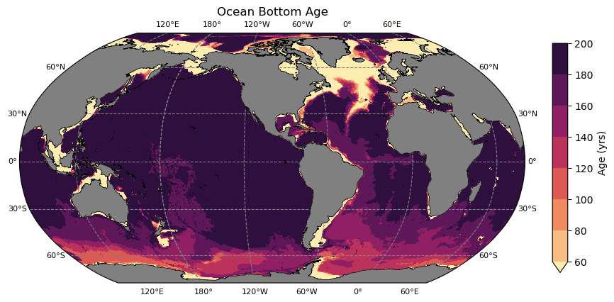
Some remarks
A few things to note here:
The continental shelves are all young - this is just because they are shallow.
The North Atlantic is also relatively young, due to formation of NADW. Note that both the Deep Western Boundary Currents and the Mid-Atlantic Ridge both sustain southward transport of this young water.
A signal following AABW pathways (northwards at the western boundaries) shows slightly younger water in these regions, but it has mixed somewhat with older water above.
Even after 200 years, the water in the NE Pacific has not experienced any ventilation…
Notes on performance
The indexing method requires the data to be loaded into memory and appears faster than it actually is if this isn’t factored in. Calculations with large datasets that do not fit within memory will struggle in this case.
The indexing method does not perform well in a dask workflow where lazy loading is being used.
The masking approach does not suffer from these limitations and when in doubt should be the preferred method. It also has the advantage of not requiring the grid data.
To illustrate this: a single month of bottom age from the original data using masking
[44]:
%%time
age.isel(time=1).where(bottom_mask).sum(dim='st_ocean').compute()
/g/data/xp65/public/apps/med_conda/envs/analysis3-26.06/lib/python3.12/site-packages/distributed/client.py:3387: UserWarning: Sending large graph of size 9.74 MiB.
This may cause some slowdown.
Consider loading the data with Dask directly
or using futures or delayed objects to embed the data into the graph without repetition.
See also https://docs.dask.org/en/stable/best-practices.html#load-data-with-dask for more information.
warnings.warn(
CPU times: user 11.5 s, sys: 4.51 s, total: 16 s
Wall time: 16.6 s
[44]:
<xarray.DataArray 'age_global' (yt_ocean: 2700, xt_ocean: 3600)> Size: 39MB
array([[0., 0., 0., ..., 0., 0., 0.],
[0., 0., 0., ..., 0., 0., 0.],
[0., 0., 0., ..., 0., 0., 0.],
...,
[0., 0., 0., ..., 0., 0., 0.],
[0., 0., 0., ..., 0., 0., 0.],
[0., 0., 0., ..., 0., 0., 0.]], shape=(2700, 3600), dtype=float32)
Coordinates:
* yt_ocean (yt_ocean) float64 22kB -81.11 -81.07 -81.02 ... 89.89 89.94 89.98
* xt_ocean (xt_ocean) float64 29kB -279.9 -279.8 -279.7 ... 79.75 79.85 79.95
time object 8B 2099-02-15 00:00:00
Attributes:
long_name: Age (global)
units: yr
valid_range: [0.e+00 1.e+20]
cell_methods: time: mean
time_avg_info: average_T1,average_T2,average_DT
standard_name: sea_water_age_since_surface_contactThe same with indexing (different month to ensure no caching effects) is significantly slower
[45]:
%%time
age.isel(time=3).isel(st_ocean=kmt).compute()
/g/data/xp65/public/apps/med_conda/envs/analysis3-26.06/lib/python3.12/site-packages/distributed/client.py:3387: UserWarning: Sending large graph of size 93.14 MiB.
This may cause some slowdown.
Consider loading the data with Dask directly
or using futures or delayed objects to embed the data into the graph without repetition.
See also https://docs.dask.org/en/stable/best-practices.html#load-data-with-dask for more information.
warnings.warn(
CPU times: user 35 s, sys: 18.9 s, total: 53.9 s
Wall time: 45.6 s
[45]:
<xarray.DataArray 'age_global' (yt_ocean: 2700, xt_ocean: 3600)> Size: 39MB
array([[nan, nan, nan, ..., nan, nan, nan],
       [nan, nan, nan, ..., nan, nan, nan],
       [nan, nan, nan, ..., nan, nan, nan],
       ...,
       [nan, nan, nan, ..., nan, nan, nan],
       [nan, nan, nan, ..., nan, nan, nan],
       [nan, nan, nan, ..., nan, nan, nan]],
      shape=(2700, 3600), dtype=float32)
Coordinates:
* yt_ocean (yt_ocean) float64 22kB -81.11 -81.07 -81.02 ... 89.89 89.94 89.98
* xt_ocean (xt_ocean) float64 29kB -279.9 -279.8 -279.7 ... 79.75 79.85 79.95
st_ocean (yt_ocean, xt_ocean) float64 78MB 0.5413 0.5413 ... 0.5413 0.5413
geolon_t (yt_ocean, xt_ocean) float32 39MB nan nan nan nan ... nan nan nan
geolat_t (yt_ocean, xt_ocean) float32 39MB nan nan nan nan ... nan nan nan
time object 8B 2099-04-16 00:00:00
Attributes:
long_name: Age (global)
units: yr
valid_range: [0.e+00 1.e+20]
cell_methods: time: mean
time_avg_info: average_T1,average_T2,average_DT
standard_name: sea_water_age_since_surface_contactIt is much faster to preload the data and then index it, but this does rely on their being sufficient memory
[46]:
%%time
myage = age.isel(time=4).load()
/g/data/xp65/public/apps/med_conda/envs/analysis3-26.06/lib/python3.12/site-packages/distributed/client.py:3387: UserWarning: Sending large graph of size 9.69 MiB.
This may cause some slowdown.
Consider loading the data with Dask directly
or using futures or delayed objects to embed the data into the graph without repetition.
See also https://docs.dask.org/en/stable/best-practices.html#load-data-with-dask for more information.
warnings.warn(
CPU times: user 33.8 s, sys: 22 s, total: 55.7 s
Wall time: 48.8 s
[47]:
%%time
myage.isel(st_ocean=kmt).compute()
CPU times: user 377 ms, sys: 99.8 ms, total: 476 ms
Wall time: 298 ms
[47]:
<xarray.DataArray 'age_global' (yt_ocean: 2700, xt_ocean: 3600)> Size: 39MB
array([[nan, nan, nan, ..., nan, nan, nan],
       [nan, nan, nan, ..., nan, nan, nan],
       [nan, nan, nan, ..., nan, nan, nan],
       ...,
       [nan, nan, nan, ..., nan, nan, nan],
       [nan, nan, nan, ..., nan, nan, nan],
       [nan, nan, nan, ..., nan, nan, nan]],
      shape=(2700, 3600), dtype=float32)
Coordinates:
* yt_ocean (yt_ocean) float64 22kB -81.11 -81.07 -81.02 ... 89.89 89.94 89.98
* xt_ocean (xt_ocean) float64 29kB -279.9 -279.8 -279.7 ... 79.75 79.85 79.95
st_ocean (yt_ocean, xt_ocean) float64 78MB 0.5413 0.5413 ... 0.5413 0.5413
geolon_t (yt_ocean, xt_ocean) float32 39MB nan nan nan nan ... nan nan nan
geolat_t (yt_ocean, xt_ocean) float32 39MB nan nan nan nan ... nan nan nan
time object 8B 2099-05-16 12:00:00
Attributes:
long_name: Age (global)
units: yr
valid_range: [0.e+00 1.e+20]
cell_methods: time: mean
time_avg_info: average_T1,average_T2,average_DT
standard_name: sea_water_age_since_surface_contact