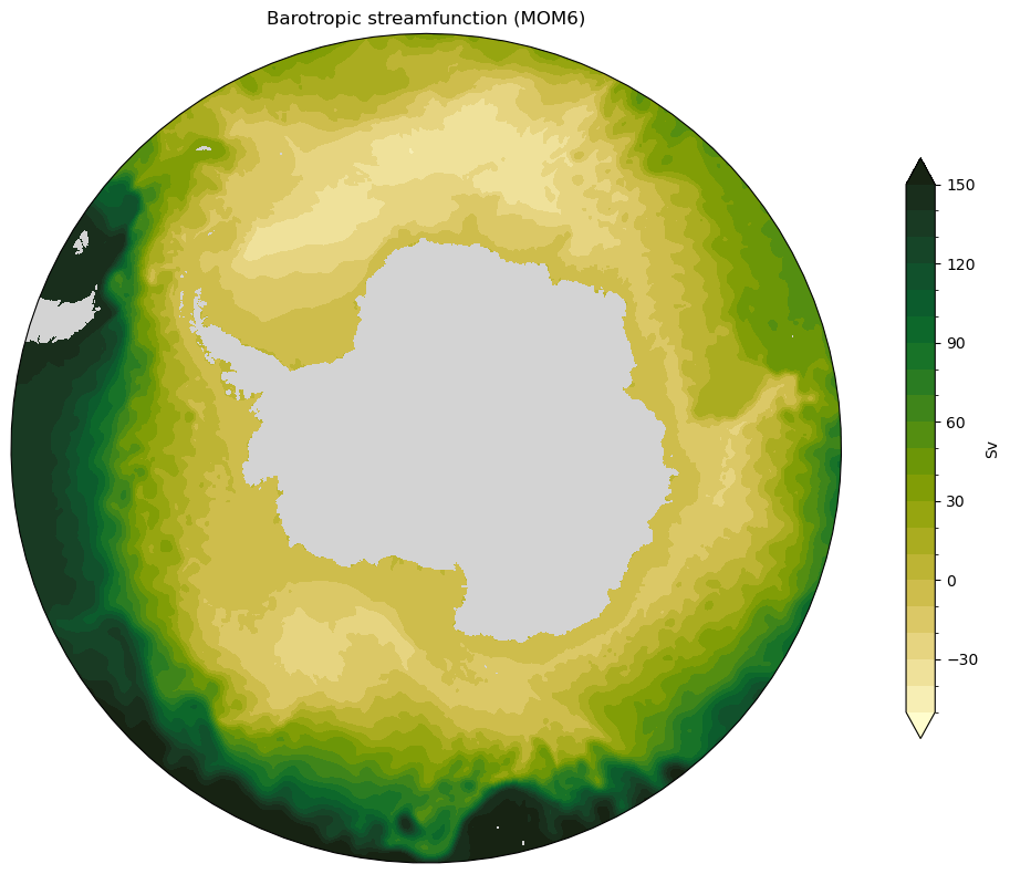
Barotropic Streamfunction
This recipe demonstrates how to compute and plot the barotropic streamfunction (\(\psi\)).
Background
The barotropic streamfunction (\(\psi\)) is obtained from the integration of the depth-integrated transports starting from a physical boundary at which we know the transport is zero - therefore there are different ways to calculate it depending on your choice of boundary for the integration.
This recipe calculates \(\psi\) integrating the depth-integrated zonal transport, \(U\) in the meridional direction, starting from the Antarctic continent:
You can see from this expression that the direction of the transport is then parallel to streamlines, and the intensity of that transport is given by the difference between streamlines. For this statement to be valid, the flow must be incompressible (or approximately so).
Requirements
This recipe uses MOM6 output.
The workflow is,
Load the MOM6 depth-integrated zonal mass transport (
umo_2d).Convert it to volume transport in Sverdrups (
Sv).Integrate meridionally (cumulative sum along latitude) to obtain the barotropic streamfunction (\(\psi\)).
Plot a circumpolar map with a circular boundary and land mask.
MOM5 adaptation
To adapt this recipe for MOM5 output, the following diagnostic equivalences may be useful:
MOM6 diagnostic (x-coord,y-coord) |
MOM5 diagnostic (x-coord,y-coord) |
|---|---|
|
|
|
|
[1]:
import cartopy.crs as ccrs
import cmocean
import intake
import matplotlib.path as mpath
import matplotlib.pyplot as plt
import numpy as np
import xarray as xr
import dask.distributed as dask
[2]:
client = dask.Client(threads_per_worker=1)
client
/g/data/xp65/public/apps/med_conda/envs/analysis3-26.06/lib/python3.12/site-packages/distributed/node.py:188: UserWarning: Port 8787 is already in use.
Perhaps you already have a cluster running?
Hosting the HTTP server on port 33711 instead
  warnings.warn(
[2]:
Client
Client-bb4ded8a-7675-11f1-88a2-0000008afe80
| Connection method: Cluster object | Cluster type: distributed.LocalCluster |
| Dashboard: /proxy/33711/status |
Cluster Info
LocalCluster
db77704a
| Dashboard: /proxy/33711/status | Workers: 48 |
| Total threads: 48 | Total memory: 188.56 GiB |
| Status: running | Using processes: True |
Scheduler Info
Scheduler
Scheduler-ccdd31cb-e445-4f17-884a-58ede0610d53
| Comm: tcp://127.0.0.1:39447 | Workers: 0 |
| Dashboard: /proxy/33711/status | Total threads: 0 |
| Started: Just now | Total memory: 0 B |
Workers
Worker: 0
| Comm: tcp://127.0.0.1:40099 | Total threads: 1 |
| Dashboard: /proxy/39657/status | Memory: 3.93 GiB |
| Nanny: tcp://127.0.0.1:32925 | |
| Local directory: /jobfs/172897319.gadi-pbs/dask-scratch-space/worker-qq85c8fz | |
Worker: 1
| Comm: tcp://127.0.0.1:32973 | Total threads: 1 |
| Dashboard: /proxy/43297/status | Memory: 3.93 GiB |
| Nanny: tcp://127.0.0.1:46673 | |
| Local directory: /jobfs/172897319.gadi-pbs/dask-scratch-space/worker-o0jl4r8a | |
Worker: 2
| Comm: tcp://127.0.0.1:33195 | Total threads: 1 |
| Dashboard: /proxy/34067/status | Memory: 3.93 GiB |
| Nanny: tcp://127.0.0.1:36497 | |
| Local directory: /jobfs/172897319.gadi-pbs/dask-scratch-space/worker-awugpj0q | |
Worker: 3
| Comm: tcp://127.0.0.1:35191 | Total threads: 1 |
| Dashboard: /proxy/45783/status | Memory: 3.93 GiB |
| Nanny: tcp://127.0.0.1:37677 | |
| Local directory: /jobfs/172897319.gadi-pbs/dask-scratch-space/worker-8tm1m3we | |
Worker: 4
| Comm: tcp://127.0.0.1:34759 | Total threads: 1 |
| Dashboard: /proxy/34195/status | Memory: 3.93 GiB |
| Nanny: tcp://127.0.0.1:39437 | |
| Local directory: /jobfs/172897319.gadi-pbs/dask-scratch-space/worker-s_n_5dbm | |
Worker: 5
| Comm: tcp://127.0.0.1:43269 | Total threads: 1 |
| Dashboard: /proxy/43095/status | Memory: 3.93 GiB |
| Nanny: tcp://127.0.0.1:39669 | |
| Local directory: /jobfs/172897319.gadi-pbs/dask-scratch-space/worker-cofkxjl9 | |
Worker: 6
| Comm: tcp://127.0.0.1:38899 | Total threads: 1 |
| Dashboard: /proxy/41627/status | Memory: 3.93 GiB |
| Nanny: tcp://127.0.0.1:44793 | |
| Local directory: /jobfs/172897319.gadi-pbs/dask-scratch-space/worker-nh2kkkuy | |
Worker: 7
| Comm: tcp://127.0.0.1:34063 | Total threads: 1 |
| Dashboard: /proxy/41293/status | Memory: 3.93 GiB |
| Nanny: tcp://127.0.0.1:40743 | |
| Local directory: /jobfs/172897319.gadi-pbs/dask-scratch-space/worker-x1cvntd8 | |
Worker: 8
| Comm: tcp://127.0.0.1:42105 | Total threads: 1 |
| Dashboard: /proxy/37375/status | Memory: 3.93 GiB |
| Nanny: tcp://127.0.0.1:39085 | |
| Local directory: /jobfs/172897319.gadi-pbs/dask-scratch-space/worker-583pbtw2 | |
Worker: 9
| Comm: tcp://127.0.0.1:41107 | Total threads: 1 |
| Dashboard: /proxy/36917/status | Memory: 3.93 GiB |
| Nanny: tcp://127.0.0.1:46431 | |
| Local directory: /jobfs/172897319.gadi-pbs/dask-scratch-space/worker-cwm6ina5 | |
Worker: 10
| Comm: tcp://127.0.0.1:35101 | Total threads: 1 |
| Dashboard: /proxy/33641/status | Memory: 3.93 GiB |
| Nanny: tcp://127.0.0.1:37667 | |
| Local directory: /jobfs/172897319.gadi-pbs/dask-scratch-space/worker-9dl39vce | |
Worker: 11
| Comm: tcp://127.0.0.1:39221 | Total threads: 1 |
| Dashboard: /proxy/36493/status | Memory: 3.93 GiB |
| Nanny: tcp://127.0.0.1:36371 | |
| Local directory: /jobfs/172897319.gadi-pbs/dask-scratch-space/worker-e0mnpede | |
Worker: 12
| Comm: tcp://127.0.0.1:43983 | Total threads: 1 |
| Dashboard: /proxy/43535/status | Memory: 3.93 GiB |
| Nanny: tcp://127.0.0.1:39863 | |
| Local directory: /jobfs/172897319.gadi-pbs/dask-scratch-space/worker-zslmyo4j | |
Worker: 13
| Comm: tcp://127.0.0.1:44883 | Total threads: 1 |
| Dashboard: /proxy/44415/status | Memory: 3.93 GiB |
| Nanny: tcp://127.0.0.1:46211 | |
| Local directory: /jobfs/172897319.gadi-pbs/dask-scratch-space/worker-wfbwh74m | |
Worker: 14
| Comm: tcp://127.0.0.1:39809 | Total threads: 1 |
| Dashboard: /proxy/42051/status | Memory: 3.93 GiB |
| Nanny: tcp://127.0.0.1:34073 | |
| Local directory: /jobfs/172897319.gadi-pbs/dask-scratch-space/worker-1h3gzw8v | |
Worker: 15
| Comm: tcp://127.0.0.1:39801 | Total threads: 1 |
| Dashboard: /proxy/32845/status | Memory: 3.93 GiB |
| Nanny: tcp://127.0.0.1:43933 | |
| Local directory: /jobfs/172897319.gadi-pbs/dask-scratch-space/worker-310fmj4z | |
Worker: 16
| Comm: tcp://127.0.0.1:44101 | Total threads: 1 |
| Dashboard: /proxy/45163/status | Memory: 3.93 GiB |
| Nanny: tcp://127.0.0.1:38531 | |
| Local directory: /jobfs/172897319.gadi-pbs/dask-scratch-space/worker-x3qhtbg8 | |
Worker: 17
| Comm: tcp://127.0.0.1:39359 | Total threads: 1 |
| Dashboard: /proxy/33999/status | Memory: 3.93 GiB |
| Nanny: tcp://127.0.0.1:43313 | |
| Local directory: /jobfs/172897319.gadi-pbs/dask-scratch-space/worker-4jn8220q | |
Worker: 18
| Comm: tcp://127.0.0.1:44015 | Total threads: 1 |
| Dashboard: /proxy/44795/status | Memory: 3.93 GiB |
| Nanny: tcp://127.0.0.1:37445 | |
| Local directory: /jobfs/172897319.gadi-pbs/dask-scratch-space/worker-97ps876c | |
Worker: 19
| Comm: tcp://127.0.0.1:35457 | Total threads: 1 |
| Dashboard: /proxy/43705/status | Memory: 3.93 GiB |
| Nanny: tcp://127.0.0.1:40397 | |
| Local directory: /jobfs/172897319.gadi-pbs/dask-scratch-space/worker-n8wfbzvt | |
Worker: 20
| Comm: tcp://127.0.0.1:35799 | Total threads: 1 |
| Dashboard: /proxy/34941/status | Memory: 3.93 GiB |
| Nanny: tcp://127.0.0.1:33527 | |
| Local directory: /jobfs/172897319.gadi-pbs/dask-scratch-space/worker-jxket5ri | |
Worker: 21
| Comm: tcp://127.0.0.1:45173 | Total threads: 1 |
| Dashboard: /proxy/45431/status | Memory: 3.93 GiB |
| Nanny: tcp://127.0.0.1:41727 | |
| Local directory: /jobfs/172897319.gadi-pbs/dask-scratch-space/worker-mc7f9t9r | |
Worker: 22
| Comm: tcp://127.0.0.1:44553 | Total threads: 1 |
| Dashboard: /proxy/44797/status | Memory: 3.93 GiB |
| Nanny: tcp://127.0.0.1:45785 | |
| Local directory: /jobfs/172897319.gadi-pbs/dask-scratch-space/worker-np4atwvq | |
Worker: 23
| Comm: tcp://127.0.0.1:34003 | Total threads: 1 |
| Dashboard: /proxy/36215/status | Memory: 3.93 GiB |
| Nanny: tcp://127.0.0.1:39383 | |
| Local directory: /jobfs/172897319.gadi-pbs/dask-scratch-space/worker-g958pw9t | |
Worker: 24
| Comm: tcp://127.0.0.1:39563 | Total threads: 1 |
| Dashboard: /proxy/41937/status | Memory: 3.93 GiB |
| Nanny: tcp://127.0.0.1:37349 | |
| Local directory: /jobfs/172897319.gadi-pbs/dask-scratch-space/worker-4dvsp3bz | |
Worker: 25
| Comm: tcp://127.0.0.1:37811 | Total threads: 1 |
| Dashboard: /proxy/36611/status | Memory: 3.93 GiB |
| Nanny: tcp://127.0.0.1:37561 | |
| Local directory: /jobfs/172897319.gadi-pbs/dask-scratch-space/worker-_afvrp1h | |
Worker: 26
| Comm: tcp://127.0.0.1:43367 | Total threads: 1 |
| Dashboard: /proxy/44929/status | Memory: 3.93 GiB |
| Nanny: tcp://127.0.0.1:45347 | |
| Local directory: /jobfs/172897319.gadi-pbs/dask-scratch-space/worker-5g2_z3qm | |
Worker: 27
| Comm: tcp://127.0.0.1:46121 | Total threads: 1 |
| Dashboard: /proxy/35555/status | Memory: 3.93 GiB |
| Nanny: tcp://127.0.0.1:39695 | |
| Local directory: /jobfs/172897319.gadi-pbs/dask-scratch-space/worker-k5prcac3 | |
Worker: 28
| Comm: tcp://127.0.0.1:43687 | Total threads: 1 |
| Dashboard: /proxy/44623/status | Memory: 3.93 GiB |
| Nanny: tcp://127.0.0.1:43735 | |
| Local directory: /jobfs/172897319.gadi-pbs/dask-scratch-space/worker-1phlxd5u | |
Worker: 29
| Comm: tcp://127.0.0.1:33097 | Total threads: 1 |
| Dashboard: /proxy/38729/status | Memory: 3.93 GiB |
| Nanny: tcp://127.0.0.1:34867 | |
| Local directory: /jobfs/172897319.gadi-pbs/dask-scratch-space/worker-34unbdy4 | |
Worker: 30
| Comm: tcp://127.0.0.1:40363 | Total threads: 1 |
| Dashboard: /proxy/37189/status | Memory: 3.93 GiB |
| Nanny: tcp://127.0.0.1:37115 | |
| Local directory: /jobfs/172897319.gadi-pbs/dask-scratch-space/worker-zeuw0oxq | |
Worker: 31
| Comm: tcp://127.0.0.1:39753 | Total threads: 1 |
| Dashboard: /proxy/37571/status | Memory: 3.93 GiB |
| Nanny: tcp://127.0.0.1:40873 | |
| Local directory: /jobfs/172897319.gadi-pbs/dask-scratch-space/worker-r9pkml2s | |
Worker: 32
| Comm: tcp://127.0.0.1:36401 | Total threads: 1 |
| Dashboard: /proxy/34001/status | Memory: 3.93 GiB |
| Nanny: tcp://127.0.0.1:41791 | |
| Local directory: /jobfs/172897319.gadi-pbs/dask-scratch-space/worker-shnmlo8v | |
Worker: 33
| Comm: tcp://127.0.0.1:37273 | Total threads: 1 |
| Dashboard: /proxy/41851/status | Memory: 3.93 GiB |
| Nanny: tcp://127.0.0.1:34409 | |
| Local directory: /jobfs/172897319.gadi-pbs/dask-scratch-space/worker-18xsrj0s | |
Worker: 34
| Comm: tcp://127.0.0.1:43565 | Total threads: 1 |
| Dashboard: /proxy/41193/status | Memory: 3.93 GiB |
| Nanny: tcp://127.0.0.1:39325 | |
| Local directory: /jobfs/172897319.gadi-pbs/dask-scratch-space/worker-kujawup7 | |
Worker: 35
| Comm: tcp://127.0.0.1:35809 | Total threads: 1 |
| Dashboard: /proxy/39007/status | Memory: 3.93 GiB |
| Nanny: tcp://127.0.0.1:34981 | |
| Local directory: /jobfs/172897319.gadi-pbs/dask-scratch-space/worker-yeplk8y3 | |
Worker: 36
| Comm: tcp://127.0.0.1:45435 | Total threads: 1 |
| Dashboard: /proxy/38507/status | Memory: 3.93 GiB |
| Nanny: tcp://127.0.0.1:37605 | |
| Local directory: /jobfs/172897319.gadi-pbs/dask-scratch-space/worker-4x5xzi75 | |
Worker: 37
| Comm: tcp://127.0.0.1:38579 | Total threads: 1 |
| Dashboard: /proxy/43517/status | Memory: 3.93 GiB |
| Nanny: tcp://127.0.0.1:46449 | |
| Local directory: /jobfs/172897319.gadi-pbs/dask-scratch-space/worker-7thsr3zp | |
Worker: 38
| Comm: tcp://127.0.0.1:46437 | Total threads: 1 |
| Dashboard: /proxy/37749/status | Memory: 3.93 GiB |
| Nanny: tcp://127.0.0.1:38083 | |
| Local directory: /jobfs/172897319.gadi-pbs/dask-scratch-space/worker-diq2fub2 | |
Worker: 39
| Comm: tcp://127.0.0.1:38605 | Total threads: 1 |
| Dashboard: /proxy/46327/status | Memory: 3.93 GiB |
| Nanny: tcp://127.0.0.1:36157 | |
| Local directory: /jobfs/172897319.gadi-pbs/dask-scratch-space/worker-ldks33sm | |
Worker: 40
| Comm: tcp://127.0.0.1:34761 | Total threads: 1 |
| Dashboard: /proxy/39617/status | Memory: 3.93 GiB |
| Nanny: tcp://127.0.0.1:35467 | |
| Local directory: /jobfs/172897319.gadi-pbs/dask-scratch-space/worker-jnc7s1cc | |
Worker: 41
| Comm: tcp://127.0.0.1:46323 | Total threads: 1 |
| Dashboard: /proxy/38001/status | Memory: 3.93 GiB |
| Nanny: tcp://127.0.0.1:44455 | |
| Local directory: /jobfs/172897319.gadi-pbs/dask-scratch-space/worker-76q3c4n3 | |
Worker: 42
| Comm: tcp://127.0.0.1:34611 | Total threads: 1 |
| Dashboard: /proxy/34255/status | Memory: 3.93 GiB |
| Nanny: tcp://127.0.0.1:33239 | |
| Local directory: /jobfs/172897319.gadi-pbs/dask-scratch-space/worker-jad2afvu | |
Worker: 43
| Comm: tcp://127.0.0.1:33885 | Total threads: 1 |
| Dashboard: /proxy/43111/status | Memory: 3.93 GiB |
| Nanny: tcp://127.0.0.1:46317 | |
| Local directory: /jobfs/172897319.gadi-pbs/dask-scratch-space/worker-bes5l9_c | |
Worker: 44
| Comm: tcp://127.0.0.1:35819 | Total threads: 1 |
| Dashboard: /proxy/39987/status | Memory: 3.93 GiB |
| Nanny: tcp://127.0.0.1:41297 | |
| Local directory: /jobfs/172897319.gadi-pbs/dask-scratch-space/worker-xevxrkni | |
Worker: 45
| Comm: tcp://127.0.0.1:46283 | Total threads: 1 |
| Dashboard: /proxy/46779/status | Memory: 3.93 GiB |
| Nanny: tcp://127.0.0.1:34345 | |
| Local directory: /jobfs/172897319.gadi-pbs/dask-scratch-space/worker-ykhuqclj | |
Worker: 46
| Comm: tcp://127.0.0.1:46291 | Total threads: 1 |
| Dashboard: /proxy/37911/status | Memory: 3.93 GiB |
| Nanny: tcp://127.0.0.1:46585 | |
| Local directory: /jobfs/172897319.gadi-pbs/dask-scratch-space/worker-bcypxc1p | |
Worker: 47
| Comm: tcp://127.0.0.1:41129 | Total threads: 1 |
| Dashboard: /proxy/39361/status | Memory: 3.93 GiB |
| Nanny: tcp://127.0.0.1:36589 | |
| Local directory: /jobfs/172897319.gadi-pbs/dask-scratch-space/worker-igxs46y3 | |
[3]:
catalog = intake.cat.access_nri
experiment = "panant-01-zstar-v13"
Load transports - use a preprocessing function to subselect a domain.
[4]:
def subset_domain(ds):
    ds = ds.sel(yh=slice(None, -50))
    return ds

umo = catalog[experiment].search(variable='umo_2d',
                                start_date='200[0,1].*',
                                frequency='1mon'
                                ).to_dask(preprocess=subset_domain)
deptho = catalog[experiment].search(variable='deptho',
                                    frequency='fx'
                                    ).to_dask(preprocess=subset_domain)
/g/data/xp65/public/apps/med_conda/envs/analysis3-26.06/lib/python3.12/site-packages/intake_esm/source.py:314: ConcatenationWarning: Attempting to concatenate datasets without valid dimension coordinates: retaining only first dataset. Request valid dimension coordinate to silence this warning.
  warnings.warn(
Take the time mean of the transport:
[5]:
mass_transport = umo['umo_2d'].mean('time')
mass_transport
[5]:
<xarray.DataArray 'umo_2d' (yh: 666, xq: 3601)> Size: 10MB
dask.array<mean_agg-aggregate, shape=(666, 3601), dtype=float32, chunksize=(666, 3601), chunktype=numpy.ndarray>
Coordinates:
  * yh       (yh) float64 5kB -81.11 -81.07 -81.02 ... -50.16 -50.09 -50.03
  * xq       (xq) float64 29kB -280.0 -279.9 -279.8 -279.7 ... 79.8 79.9 80.0
Attributes:
    units:          kg s-1
    long_name:      Ocean Mass X Transport Vertical Sum
    cell_methods:   yh:sum xq:point time: mean
    time_avg_info:  average_T1,average_T2,average_DT
    standard_name:  ocean_mass_x_transport_vertical_sum
interp_method: noneLooking at the mass_transport attributes, we can confirm that it is a mass transport from its units. To convert to volume transoprt we need to divide by the reference density.
[6]:
ρ0 = 1030  # reference seawater density, kg m⁻³
volume_transport = mass_transport / ρ0   # convert kg s⁻¹ -> m³ s⁻¹
To integrate the transport in the meridional direction, we just need to sum cumulatively northwards - this is because the transport is the total amount of water through a grid face.
We also divide by 1e6 to convert from m³ s⁻¹ to Sv (1 Sv = 10⁶ m³ s⁻¹)
[7]:
psi = volume_transport.cumsum('yh') / 1e6 # convert m³ s⁻¹ -> Sv
Now lets create a land mask for plotting:
[8]:
land_mask = xr.where(np.isnan(deptho['deptho']), 1, np.nan)
[9]:
fig = plt.figure(figsize=(12, 8))
ax = plt.axes(projection=ccrs.SouthPolarStereo())
ax.set_extent([-180, 180, -80, -50], crs=ccrs.PlateCarree())
ax.set_facecolor('lightgrey')

# Map the plot boundaries to a circle
theta = np.linspace(0, 2 * np.pi, 100)
center, radius = [0.5, 0.5], 0.5
verts = np.vstack([np.sin(theta), np.cos(theta)]).T
circle = mpath.Path(verts * radius + center)
ax.set_boundary(circle, transform=ax.transAxes)

psi.plot.contourf(ax=ax,
                  levels=np.arange(-50, 160, 10),
                  extend='both',
                  cmap=cmocean.cm.speed,
                  cbar_kwargs={'shrink':.7, 'label':'Sv'},
                  transform=ccrs.PlateCarree())

land_mask.plot.contourf(ax=ax,
                        colors=['lightgrey'],
                        add_colorbar=False,
                        transform=ccrs.PlateCarree())


plt.title("Barotropic streamfunction (MOM6)")
plt.tight_layout()