Using cf_xarray and pint for Model Agnostic Analysis
Introduction
In this Advanced tutorial, we learn how cf_xarray and pint can be used for model-agnostic analysis. This means writing your notebook so that it can easily be used with any CF-compliant data source.
Background: COSIMA Recipes once included model-agnostic analysis in many of the example recipes to support both ACCESS-OM2/MOM5 and MOM6 analysis. However, this made some recipes difficult to read and understand because it obscured grid or variable information, which are important for users to learn. Most COSIMA Recipes now take a pedagogical approach and show an example of analysis for one model, with some additional information on how a user might modify the recipe for a different model,
for example, the equivalent variable names. Users who wish to perform model-agnostic analysis may find this cf_xarray and pint tutorial helpful!
What are the CF Conventions?
From CF Metadata conventions:
The CF metadata conventions are designed to promote the processing and sharing of files created with the NetCDF API. The conventions define metadata that provide a definitive description of what the data in each variable represents, and the spatial and temporal properties of the data. This enables users of data from different sources to decide which quantities are comparable, and facilitates building applications with powerful extraction, regridding, and display capabilities. The CF convention includes a standard name table, which defines strings that identify physical quantities.
In most cases the model output data accessed through the ACCESS-NRI Intake Catalog complies with some version of the CF conventions; enough to be usable for model agnostic analysis.
Why bother?
Model agnostic means the same code can work for multiple models. This makes your code more usable by you and by others. You no longer need to have different versions of code for different models. It makes you and any one who uses your code more productive. It allows for common tasks to be abstracted into general methods that can be more easily reused, meaning less code needs to be written and maintained. This is an enormous productivity boost.
How is model agnostic analysis achieved?
This can be achieved by using packages that enable this:
cf_xarray for generalised coordinate naming
xgcm to make grid operations generic across data
pint and pint-xarray for handling units easily and robustly
Example
Introduction
This tutorial uses an example analysis, shows how the this might be done in a traditional, model specific, manner, and then implements the same analysis in a model agnostic way.
This tutorial is intended to be run using the conda/analysis3 or conda/access-med environment, available via the xp65 project: https://access-nri-intake-catalog.readthedocs.io/en/latest/usage/how.html#using-the-catalog-on-the-are
The first step is to import necessary packages.
[1]:
import intake

import numpy as np
import xarray as xr
import cf_xarray as cfxr
import pint_xarray

from pint import application_registry as ureg
import cf_xarray.units
import matplotlib.pyplot as plt
import cmocean as cm
import cartopy.crs as ccrs
import cartopy.feature as cft
[2]:
from dask.distributed import Client
client = Client(threads_per_worker=1)
client
/g/data/xp65/public/apps/med_conda/envs/analysis3-26.06/lib/python3.12/site-packages/distributed/node.py:188: UserWarning: Port 8787 is already in use.
Perhaps you already have a cluster running?
Hosting the HTTP server on port 45243 instead
  warnings.warn(
[2]:
Client
Client-94a5f54f-7517-11f1-a646-000003d5fe80
| Connection method: Cluster object | Cluster type: distributed.LocalCluster |
| Dashboard: /proxy/45243/status |
Cluster Info
LocalCluster
d38ffbf4
| Dashboard: /proxy/45243/status | Workers: 28 |
| Total threads: 28 | Total memory: 251.19 GiB |
| Status: running | Using processes: True |
Scheduler Info
Scheduler
Scheduler-7c6c47d3-f8d3-4720-85d6-56bedbcb303d
| Comm: tcp://127.0.0.1:40435 | Workers: 0 |
| Dashboard: /proxy/45243/status | Total threads: 0 |
| Started: Just now | Total memory: 0 B |
Workers
Worker: 0
| Comm: tcp://127.0.0.1:41303 | Total threads: 1 |
| Dashboard: /proxy/34983/status | Memory: 8.97 GiB |
| Nanny: tcp://127.0.0.1:39017 | |
| Local directory: /jobfs/172757805.gadi-pbs/dask-scratch-space/worker-urs7g1oi | |
Worker: 1
| Comm: tcp://127.0.0.1:39779 | Total threads: 1 |
| Dashboard: /proxy/36401/status | Memory: 8.97 GiB |
| Nanny: tcp://127.0.0.1:33315 | |
| Local directory: /jobfs/172757805.gadi-pbs/dask-scratch-space/worker-w3xfxem8 | |
Worker: 2
| Comm: tcp://127.0.0.1:40589 | Total threads: 1 |
| Dashboard: /proxy/45529/status | Memory: 8.97 GiB |
| Nanny: tcp://127.0.0.1:41563 | |
| Local directory: /jobfs/172757805.gadi-pbs/dask-scratch-space/worker-cberydql | |
Worker: 3
| Comm: tcp://127.0.0.1:42511 | Total threads: 1 |
| Dashboard: /proxy/46621/status | Memory: 8.97 GiB |
| Nanny: tcp://127.0.0.1:43273 | |
| Local directory: /jobfs/172757805.gadi-pbs/dask-scratch-space/worker-0selp0le | |
Worker: 4
| Comm: tcp://127.0.0.1:40511 | Total threads: 1 |
| Dashboard: /proxy/38341/status | Memory: 8.97 GiB |
| Nanny: tcp://127.0.0.1:43073 | |
| Local directory: /jobfs/172757805.gadi-pbs/dask-scratch-space/worker-yat3eelt | |
Worker: 5
| Comm: tcp://127.0.0.1:34377 | Total threads: 1 |
| Dashboard: /proxy/41529/status | Memory: 8.97 GiB |
| Nanny: tcp://127.0.0.1:34527 | |
| Local directory: /jobfs/172757805.gadi-pbs/dask-scratch-space/worker-lzla5qun | |
Worker: 6
| Comm: tcp://127.0.0.1:35525 | Total threads: 1 |
| Dashboard: /proxy/45515/status | Memory: 8.97 GiB |
| Nanny: tcp://127.0.0.1:45927 | |
| Local directory: /jobfs/172757805.gadi-pbs/dask-scratch-space/worker-drvdn45t | |
Worker: 7
| Comm: tcp://127.0.0.1:42791 | Total threads: 1 |
| Dashboard: /proxy/36801/status | Memory: 8.97 GiB |
| Nanny: tcp://127.0.0.1:43591 | |
| Local directory: /jobfs/172757805.gadi-pbs/dask-scratch-space/worker-asgdphq9 | |
Worker: 8
| Comm: tcp://127.0.0.1:37953 | Total threads: 1 |
| Dashboard: /proxy/37303/status | Memory: 8.97 GiB |
| Nanny: tcp://127.0.0.1:43529 | |
| Local directory: /jobfs/172757805.gadi-pbs/dask-scratch-space/worker-gan6ka40 | |
Worker: 9
| Comm: tcp://127.0.0.1:44679 | Total threads: 1 |
| Dashboard: /proxy/43331/status | Memory: 8.97 GiB |
| Nanny: tcp://127.0.0.1:44451 | |
| Local directory: /jobfs/172757805.gadi-pbs/dask-scratch-space/worker-us_bocez | |
Worker: 10
| Comm: tcp://127.0.0.1:45281 | Total threads: 1 |
| Dashboard: /proxy/45949/status | Memory: 8.97 GiB |
| Nanny: tcp://127.0.0.1:41085 | |
| Local directory: /jobfs/172757805.gadi-pbs/dask-scratch-space/worker-f86qzind | |
Worker: 11
| Comm: tcp://127.0.0.1:37907 | Total threads: 1 |
| Dashboard: /proxy/33337/status | Memory: 8.97 GiB |
| Nanny: tcp://127.0.0.1:45767 | |
| Local directory: /jobfs/172757805.gadi-pbs/dask-scratch-space/worker-aqwwpl9_ | |
Worker: 12
| Comm: tcp://127.0.0.1:34415 | Total threads: 1 |
| Dashboard: /proxy/41907/status | Memory: 8.97 GiB |
| Nanny: tcp://127.0.0.1:45545 | |
| Local directory: /jobfs/172757805.gadi-pbs/dask-scratch-space/worker-ktc98tpg | |
Worker: 13
| Comm: tcp://127.0.0.1:44509 | Total threads: 1 |
| Dashboard: /proxy/43911/status | Memory: 8.97 GiB |
| Nanny: tcp://127.0.0.1:39675 | |
| Local directory: /jobfs/172757805.gadi-pbs/dask-scratch-space/worker-4ltl638s | |
Worker: 14
| Comm: tcp://127.0.0.1:40515 | Total threads: 1 |
| Dashboard: /proxy/34233/status | Memory: 8.97 GiB |
| Nanny: tcp://127.0.0.1:41255 | |
| Local directory: /jobfs/172757805.gadi-pbs/dask-scratch-space/worker-6tvlj0yo | |
Worker: 15
| Comm: tcp://127.0.0.1:43629 | Total threads: 1 |
| Dashboard: /proxy/41697/status | Memory: 8.97 GiB |
| Nanny: tcp://127.0.0.1:33305 | |
| Local directory: /jobfs/172757805.gadi-pbs/dask-scratch-space/worker-9gzpi2oq | |
Worker: 16
| Comm: tcp://127.0.0.1:44703 | Total threads: 1 |
| Dashboard: /proxy/44867/status | Memory: 8.97 GiB |
| Nanny: tcp://127.0.0.1:40119 | |
| Local directory: /jobfs/172757805.gadi-pbs/dask-scratch-space/worker-vtgzqwuf | |
Worker: 17
| Comm: tcp://127.0.0.1:45719 | Total threads: 1 |
| Dashboard: /proxy/45127/status | Memory: 8.97 GiB |
| Nanny: tcp://127.0.0.1:33479 | |
| Local directory: /jobfs/172757805.gadi-pbs/dask-scratch-space/worker-nuubmntk | |
Worker: 18
| Comm: tcp://127.0.0.1:42801 | Total threads: 1 |
| Dashboard: /proxy/39187/status | Memory: 8.97 GiB |
| Nanny: tcp://127.0.0.1:40637 | |
| Local directory: /jobfs/172757805.gadi-pbs/dask-scratch-space/worker-z3yz6hqg | |
Worker: 19
| Comm: tcp://127.0.0.1:36979 | Total threads: 1 |
| Dashboard: /proxy/45861/status | Memory: 8.97 GiB |
| Nanny: tcp://127.0.0.1:38117 | |
| Local directory: /jobfs/172757805.gadi-pbs/dask-scratch-space/worker-azlhjz1o | |
Worker: 20
| Comm: tcp://127.0.0.1:39477 | Total threads: 1 |
| Dashboard: /proxy/36991/status | Memory: 8.97 GiB |
| Nanny: tcp://127.0.0.1:41727 | |
| Local directory: /jobfs/172757805.gadi-pbs/dask-scratch-space/worker-iqf7iieu | |
Worker: 21
| Comm: tcp://127.0.0.1:40033 | Total threads: 1 |
| Dashboard: /proxy/39597/status | Memory: 8.97 GiB |
| Nanny: tcp://127.0.0.1:36403 | |
| Local directory: /jobfs/172757805.gadi-pbs/dask-scratch-space/worker-jzeluvhx | |
Worker: 22
| Comm: tcp://127.0.0.1:39605 | Total threads: 1 |
| Dashboard: /proxy/42133/status | Memory: 8.97 GiB |
| Nanny: tcp://127.0.0.1:34809 | |
| Local directory: /jobfs/172757805.gadi-pbs/dask-scratch-space/worker-20oylny6 | |
Worker: 23
| Comm: tcp://127.0.0.1:35845 | Total threads: 1 |
| Dashboard: /proxy/34891/status | Memory: 8.97 GiB |
| Nanny: tcp://127.0.0.1:36815 | |
| Local directory: /jobfs/172757805.gadi-pbs/dask-scratch-space/worker-hz_lcj5g | |
Worker: 24
| Comm: tcp://127.0.0.1:35889 | Total threads: 1 |
| Dashboard: /proxy/34713/status | Memory: 8.97 GiB |
| Nanny: tcp://127.0.0.1:44871 | |
| Local directory: /jobfs/172757805.gadi-pbs/dask-scratch-space/worker-x8m9newa | |
Worker: 25
| Comm: tcp://127.0.0.1:40867 | Total threads: 1 |
| Dashboard: /proxy/40475/status | Memory: 8.97 GiB |
| Nanny: tcp://127.0.0.1:42041 | |
| Local directory: /jobfs/172757805.gadi-pbs/dask-scratch-space/worker-td3oyun_ | |
Worker: 26
| Comm: tcp://127.0.0.1:40831 | Total threads: 1 |
| Dashboard: /proxy/42655/status | Memory: 8.97 GiB |
| Nanny: tcp://127.0.0.1:35005 | |
| Local directory: /jobfs/172757805.gadi-pbs/dask-scratch-space/worker-penmd13g | |
Worker: 27
| Comm: tcp://127.0.0.1:40817 | Total threads: 1 |
| Dashboard: /proxy/44247/status | Memory: 8.97 GiB |
| Nanny: tcp://127.0.0.1:46611 | |
| Local directory: /jobfs/172757805.gadi-pbs/dask-scratch-space/worker-3bgzzc1v | |
cf_xarray works best when xarray keeps attributes by default:
[3]:
xr.set_options(keep_attrs=True)
[3]:
<xarray.core.options.set_options at 0x154ac4a22360>
Load the ACCESS-NRI Intake Catalog:
[4]:
catalog = intake.cat.access_nri
Then, select one experiment from the catalog and load surface temperature data from a 0.25\(^\circ\) global MOM5 model.
[5]:
experiment = '025deg_jra55_iaf_omip2_cycle6'
cat_subset = catalog[experiment]

variable = 'sst'
var_search = cat_subset.search(variable=variable, frequency='1mon')
ds = var_search.to_dask(xarray_open_kwargs={
    # This option suppresses a warning due to an upcoming default alteration in xarray
    "decode_timedelta": False,
})
SST = ds[variable]
This is a 3D dataset in latitude, longitude and time:
[6]:
SST
[6]:
<xarray.DataArray 'sst' (time: 732, yt_ocean: 1080, xt_ocean: 1440)> Size: 5GB
dask.array<concatenate, shape=(732, 1080, 1440), dtype=float32, chunksize=(12, 1080, 1440), chunktype=numpy.ndarray>
Coordinates:
  * time      (time) datetime64[ns] 6kB 1958-01-14T12:00:00 ... 2018-12-14T12...
  * yt_ocean  (yt_ocean) float64 9kB -81.08 -80.97 -80.87 ... 89.74 89.84 89.95
  * xt_ocean  (xt_ocean) float64 12kB -279.9 -279.6 -279.4 ... 79.38 79.62 79.88
Attributes:
    long_name:      Potential temperature
    units:          K
    valid_range:    [-10. 500.]
    cell_methods:   time: mean
    time_avg_info:  average_T1,average_T2,average_DT
standard_name: sea_surface_temperatureModel specific
First, do our analysis as it might usually be done, in a model-specific manner:
Convert the temperature units from kelvin (K) to Celsius (C);
Use the time coordinate name in the mean function.
We use pint to ensure this is in degrees C. Note that if the data were originally in degrees Celcius, this would do nothing. This is a way of catering for any temperature units that are understood by pint in a transparent way. Note the call to quantify, which invokes pint’s machinery to parse the units and allow unit conversions.
[7]:
SST.attrs['units'] = 'K'
SST = SST.pint.quantify().pint.to('C')
SST_time_mean = SST.mean('time')
SST_time_mean
[7]:
<xarray.DataArray 'sst' (yt_ocean: 1080, xt_ocean: 1440)> Size: 6MB
<Quantity(dask.array<mean_agg-aggregate, shape=(1080, 1440), dtype=float32, chunksize=(1080, 1440), chunktype=numpy.ndarray>, 'degree_Celsius')>
Coordinates:
  * yt_ocean  (yt_ocean) float64 9kB [degrees_north] -81.08 -80.97 ... 89.95
  * xt_ocean  (xt_ocean) float64 12kB [degrees_east] -279.9 -279.6 ... 79.88
Indexes:
    xt_ocean  PintIndex(PandasIndex, units={'xt_ocean': 'degrees_east'})
    yt_ocean  PintIndex(PandasIndex, units={'yt_ocean': 'degrees_north'})
Attributes:
    long_name:      Potential temperature
    valid_range:    [-10. 500.]
    cell_methods:   time: mean
    time_avg_info:  average_T1,average_T2,average_DT
standard_name: sea_surface_temperatureNow, plot the result:
[8]:
plt.figure(figsize=(12, 6))
ax = plt.axes(projection=ccrs.Robinson())

SST_time_mean = SST_time_mean.pint.dequantify()
SST_time_mean.plot(ax=ax,
                   x='xt_ocean', y='yt_ocean',
                   transform=ccrs.PlateCarree(),
                   vmin=-2, vmax=30, extend='both',
                   cmap=cm.cm.thermal)

ax.coastlines()
[8]:
<cartopy.mpl.feature_artist.FeatureArtist at 0x15486dbcacc0>
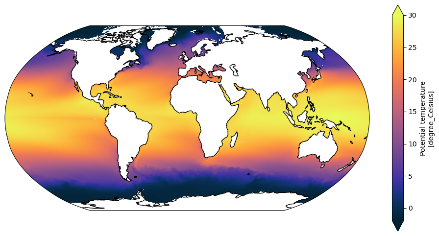
(Note that the Arctic is not correctly respresented due to the 1D lat/lon coordinates not being correct in the tripole area. See the Making Maps with cartopy Tutorial for more information.)
Model agnostic
Now, do the same calculation, but in a model agnostic manner.
We can use the cf accessor to automatically determine the name of the time dimension without knowledge of the exact model being used. cf_xarray checks the names of variables and coordinates, and associated metadata, to try and infer information about the data based on the CF conventions.
To see what cf_xarray information is available just evaluate the accessor:
[9]:
SST.cf
[9]:
Coordinates:
             CF Axes: * X: ['xt_ocean']
                      * Y: ['yt_ocean']
                      * T: ['time']
                        Z: n/a

      CF Coordinates: * longitude: ['xt_ocean']
                      * latitude: ['yt_ocean']
                      * time: ['time']
                        vertical: n/a

       Cell Measures:   area, volume: n/a

      Standard Names:   n/a

              Bounds:   n/a

       Grid Mappings:   n/a
In this case it has found X, Y and T axes, and longitude, latitude and time coordinates. These are now accessible like a dict using the cf accessor. Note that this returns the actual coordinate, and many functions just want a simple string argument, which is the name of the coordinate.
cf_xarray also wraps many standard xarray functions, allowing cf names to be used, which are automatically converted to the name in the data.
The upshot: just use the cf accessor, append the required function, and use the standard CF coordinate name (in this case they are the same, time, but that is not guaranteed):
[10]:
SST_time_mean = SST.cf.mean('time')
SST_time_mean
[10]:
<xarray.DataArray 'sst' (yt_ocean: 1080, xt_ocean: 1440)> Size: 6MB
<Quantity(dask.array<mean_agg-aggregate, shape=(1080, 1440), dtype=float32, chunksize=(1080, 1440), chunktype=numpy.ndarray>, 'degree_Celsius')>
Coordinates:
  * yt_ocean  (yt_ocean) float64 9kB [degrees_north] -81.08 -80.97 ... 89.95
  * xt_ocean  (xt_ocean) float64 12kB [degrees_east] -279.9 -279.6 ... 79.88
Indexes:
    xt_ocean  PintIndex(PandasIndex, units={'xt_ocean': 'degrees_east'})
    yt_ocean  PintIndex(PandasIndex, units={'yt_ocean': 'degrees_north'})
Attributes:
    long_name:      Potential temperature
    valid_range:    [-10. 500.]
    cell_methods:   time: mean
    time_avg_info:  average_T1,average_T2,average_DT
standard_name: sea_surface_temperatureUsing the cf_xarray-wrapped function makes the code more legible and easier to write, i.e.
SST.cf.mean('time')
compared to
SST.mean(SST.cf['time'].name)
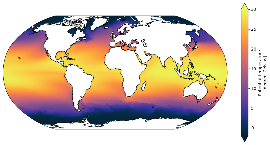
The cf accessor can be used in the same way in the plot, with the CF names for latitude and longitude used as x and y arguments:
[11]:
plt.figure(figsize=(12, 6))
ax = plt.axes(projection=ccrs.Robinson())

SST_time_mean = SST_time_mean.pint.dequantify()
SST_time_mean.cf.plot(ax=ax,
                      x='longitude', y='latitude',
                      transform=ccrs.PlateCarree(),
                      vmin=-2, vmax=30, extend='both',
                      cmap=cm.cm.thermal)

ax.coastlines()
[11]:
<cartopy.mpl.feature_artist.FeatureArtist at 0x154806240230>
Putting this into practice
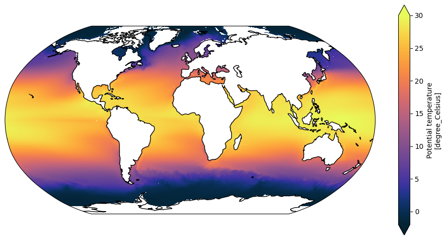
Above a model agnostic version of some code was demonstrated, but that doesn’t utilise the full power of what it is capable of. The model agnostic code can now be easily turned into a function that accepts an xarray DataArray:
[12]:
def map_mean_temp_in_degrees_celsius(da):
    # Take the time mean of da and plot a global temperature field in a Robinson projection
    #
    # Input DataArray (da) should be a 3D array of latitude, longitude and time.

    da = da.pint.quantify().pint.to('C')
    da_time_mean = da.cf.mean('time')

    plt.figure(figsize=(12, 6))
    ax = plt.axes(projection=ccrs.Robinson())

    da_time_mean = da_time_mean.pint.dequantify()
    da_time_mean.cf.plot(ax=ax,
                         x='longitude', y='latitude',
                         transform=ccrs.PlateCarree(),
                         vmin=-2, vmax=30, extend='both',
                         cmap=cm.cm.thermal)

    ax.coastlines()
Try this out with the SST data used above:
[13]:
map_mean_temp_in_degrees_celsius(SST)
Now try on the output from a different experiment and model (MOM6):
[14]:
experiment = 'OM4_025.JRA_RYF'
variable = 'tos'
cat_subset = catalog[experiment]
var_search = cat_subset.search(variable=variable, frequency='1mon')
ds = var_search.to_dask(xarray_open_kwargs={"decode_timedelta": False})
SST_mom6 = ds[variable]
/jobfs/172757805.gadi-pbs/ipykernel_3614278/3257732426.py:4: UserWarning: Value aliasing: variable='tos' → variable=['('surface_temp',)','tos']
  var_search = cat_subset.search(variable=variable, frequency='1mon')
Check to see it has correctly parsed the CF information. It is not necessary to print this out, but interesting, and note it has quite different index and coordinate names
[15]:
SST_mom6.cf
[15]:
Coordinates:
             CF Axes: * X: ['xh']
                      * Y: ['yh']
                      * T: ['time']
                        Z: n/a

      CF Coordinates: * longitude: ['xh']
                      * latitude: ['yh']
                      * time: ['time']
                        vertical: n/a

       Cell Measures:   area, volume: n/a

      Standard Names:   n/a

              Bounds:   n/a

       Grid Mappings:   n/a
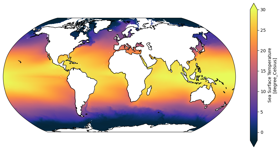
Use the function from above which also worked on MOM5 data with very different coordinates
[16]:
map_mean_temp_in_degrees_celsius(SST_mom6)
What to do when it goes wrong
The model agnostic function worked flawlessly with two different ocean data sets, after the units were corrected in the MOM5 data. What about some ice data?
Using the same experiment from which the first SST data was obtained, load the ice air temperature variable:
[17]:
catalog.search(name=".*025deg", realm="seaIce", variable="Tair_m")
Intake dataframe catalog with 12 source(s) across 12 rows:
| model | description | realm | frequency | variable | |
|---|---|---|---|---|---|
| name | |||||
| 025deg_era5_iaf | {ACCESS-OM2} | {0.25 degree ACCESS-OM2 global model configuration with ERA5 interannual\nforcing (1980-2021)} | {seaIce} | {1mon} | {Tair_m} |
| 025deg_era5_ryf | {ACCESS-OM2} | {0.25 degree ACCESS-OM2 global model configuration with ERA5 RYF9091 repeat\nyear forcing (May 1990 to Apr 1991)} | {seaIce} | {1mon} | {Tair_m} |
| 025deg_jra55_iaf_cycle6_online_mlt | {ACCESS-OM2} | {ACCESS-OM2 0.25 degree interannual forcing simulation with mixed layer tracer budget diagnostics} | {seaIce} | {1mon} | {Tair_m} |
| 025deg_jra55_iaf_era5comparison | {ACCESS-OM2} | {0.25 degree ACCESS-OM2 global model configuration with JRA55-do v1.5.0\ninterannual forcing (1980-2019)} | {seaIce} | {1mon} | {Tair_m} |
| 025deg_jra55_iaf_omip2_cycle1 | {ACCESS-OM2} | {Cycle 1/6 of 0.25 degree ACCESS-OM2 physics-only global configuration with JRA55-do v1.4 OMIP2 interannual forcing (1958-2019)} | {seaIce} | {1mon} | {Tair_m} |
| 025deg_jra55_iaf_omip2_cycle2 | {ACCESS-OM2} | {Cycle 1/6 of 0.25 degree ACCESS-OM2 physics-only global configuration with JRA55-do v1.4 OMIP2 interannual forcing (1958-2019)} | {seaIce} | {1mon} | {Tair_m} |
| 025deg_jra55_iaf_omip2_cycle3 | {ACCESS-OM2} | {Cycle 3/6 of 0.25 degree ACCESS-OM2 physics-only global configuration with JRA55-do v1.4 OMIP2 interannual forcing (1958-2019)} | {seaIce} | {1mon} | {Tair_m} |
| 025deg_jra55_iaf_omip2_cycle4 | {ACCESS-OM2} | {Cycle 4/6 of 0.25 degree ACCESS-OM2 physics-only global configuration with JRA55-do v1.4 OMIP2 interannual forcing (1958-2019)} | {seaIce} | {1mon} | {Tair_m} |
| 025deg_jra55_iaf_omip2_cycle5 | {ACCESS-OM2} | {Cycle 5/6 of 0.25 degree ACCESS-OM2 physics-only global configuration with JRA55-do v1.4 OMIP2 interannual forcing (1958-2019)} | {seaIce} | {1mon} | {Tair_m} |
| 025deg_jra55_iaf_omip2_cycle6 | {ACCESS-OM2} | {Cycle 6/6 of 0.25 degree ACCESS-OM2 physics-only global configuration with JRA55-do v1.4 OMIP2 interannual forcing (1958-2019)} | {seaIce} | {1mon} | {Tair_m} |
| 025deg_jra55_ryf9091_gadi | {ACCESS-OM2} | {0.25 degree ACCESS-OM2 physics-only global configuration with JRA55-do v1.3 RYF9091 repeat year forcing (May 1990 to Apr 1991)} | {seaIce} | {1mon} | {Tair_m} |
| 025deg_jra55_ryf_era5comparison | {ACCESS-OM2} | {0.25 degree ACCESS-OM2 global model configuration with JRA55-do v1.4.0\nRYF9091 repeat year forcing (May 1990 to Apr 1991)} | {seaIce} | {1mon} | {Tair_m} |
[18]:
experiment = "025deg_jra55_iaf_omip2_cycle6"
variable = 'Tair_m'
cat_subset = catalog[experiment]
var_search = cat_subset.search(variable=variable, frequency='1mon')
ds = var_search.to_dask(
    xarray_open_kwargs={"decode_timedelta": False},
    # xarray_combine_by_coords_kwargs is required to get the
    # data from this experiment loaded in a reasonable timeframe
    xarray_combine_by_coords_kwargs = dict(
    compat="override",
    data_vars="minimal",
    coords="minimal",
),
)
ice_air_temp = ds[variable]
ice_air_temp
[18]:
<xarray.DataArray 'Tair_m' (time: 732, nj: 1080, ni: 1440)> Size: 5GB
dask.array<concatenate, shape=(732, 1080, 1440), dtype=float32, chunksize=(1, 1080, 1440), chunktype=numpy.ndarray>
Coordinates:
  * time     (time) datetime64[ns] 6kB 1958-02-01 1958-03-01 ... 2019-01-01
    TLON     (nj, ni) float32 6MB dask.array<chunksize=(1080, 1440), meta=np.ndarray>
    TLAT     (nj, ni) float32 6MB dask.array<chunksize=(1080, 1440), meta=np.ndarray>
    ULON     (nj, ni) float32 6MB dask.array<chunksize=(1080, 1440), meta=np.ndarray>
    ULAT     (nj, ni) float32 6MB dask.array<chunksize=(1080, 1440), meta=np.ndarray>
Dimensions without coordinates: nj, ni
Attributes:
    units:          C
    long_name:      air temperature
    cell_measures:  area: tarea
    cell_methods:   time: mean
time_rep: averagedWhen we try the generic routine:
[19]:
map_mean_temp_in_degrees_celsius(ice_air_temp)
---------------------------------------------------------------------------
KeyError                                  Traceback (most recent call last)
Cell In[19], line 1
----> 1 map_mean_temp_in_degrees_celsius(ice_air_temp)

Cell In[12], line 13, in map_mean_temp_in_degrees_celsius(da)
      9     plt.figure(figsize=(12, 6))
     10     ax = plt.axes(projection=ccrs.Robinson())
     11
     12     da_time_mean = da_time_mean.pint.dequantify()
---> 13     da_time_mean.cf.plot(ax=ax,
     14                          x='longitude', y='latitude',
     15                          transform=ccrs.PlateCarree(),
     16                          vmin=-2, vmax=30, extend='both',

File /g/data/xp65/public/apps/med_conda/envs/analysis3-26.06/lib/python3.12/site-packages/cf_xarray/accessor.py:1451, in _CFWrappedPlotMethods.__call__(self, *args, **kwargs)
   1442 """
   1443 Allows .plot()
   1444 """
   1445 plot = _getattr(
   1446     obj=self._obj,
   1447     attr="plot",
   1448     accessor=self.accessor,
   1449     key_mappers=dict.fromkeys(self._keys, (_single(_get_all),)),
   1450 )
-> 1451 return self._plot_decorator(plot)(*args, **kwargs)

File /g/data/xp65/public/apps/med_conda/envs/analysis3-26.06/lib/python3.12/site-packages/cf_xarray/accessor.py:1434, in _CFWrappedPlotMethods._plot_decorator.<locals>._plot_wrapper(*args, **kwargs)
   1431     kwargs = self._process_x_or_y(kwargs, "y", skip=kwargs.get("x"))
   1433 # Now set some nice properties
-> 1434 kwargs = self._set_axis_props(kwargs, "x")
   1435 kwargs = self._set_axis_props(kwargs, "y")
   1437 return func(*args, **kwargs)

File /g/data/xp65/public/apps/med_conda/envs/analysis3-26.06/lib/python3.12/site-packages/cf_xarray/accessor.py:1398, in _CFWrappedPlotMethods._set_axis_props(self, kwargs, key)
   1396 if value:
   1397     if value in self.accessor.keys():
-> 1398         var = self.accessor[value]
   1399     else:
   1400         var = self._obj[value]

File /g/data/xp65/public/apps/med_conda/envs/analysis3-26.06/lib/python3.12/site-packages/cf_xarray/accessor.py:3472, in CFDataArrayAccessor.__getitem__(self, key)
   3467 if not isinstance(key, Hashable):
   3468     raise KeyError(
   3469         f"Cannot use an Iterable of keys with DataArrays. Expected a single string. Received {key!r} instead."
   3470     )
-> 3472 return _getitem(self, key)

File /g/data/xp65/public/apps/med_conda/envs/analysis3-26.06/lib/python3.12/site-packages/cf_xarray/accessor.py:1184, in _getitem(accessor, key, skip)
   1182 names = _get_all(obj, k)
   1183 names = drop_bounds(names)
-> 1184 check_results(names, k)
   1185 successful[k] = bool(names)
   1186 coords.extend(names)

File /g/data/xp65/public/apps/med_conda/envs/analysis3-26.06/lib/python3.12/site-packages/cf_xarray/accessor.py:1124, in _getitem.<locals>.check_results(names, key)
   1122 def check_results(names, key):
   1123     if scalar_key and len(names) > 1:
-> 1124         raise KeyError(
   1125             f"Receive multiple variables for key {key!r}: {names}. "
   1126             f"Expected only one. Please pass a list [{key!r}] "
   1127             f"instead to get all variables matching {key!r}."
   1128         )

KeyError: "Receive multiple variables for key 'longitude': ['TLON', 'ULON']. Expected only one. Please pass a list ['longitude'] instead to get all variables matching 'longitude'."

The error message is
"Receive multiple variables for key 'longitude': ['TLON', 'ULON']. Expected only one. Please pass a list ['longitude'] instead to get all variables matching 'longitude'."
This suggests that cf_xarray has found multiple longitude coordinates TLON and ULON and doesn’t know how to resolve this automatically.
Inspecting the cf information doesn’t show multiple axes like it does in the documentation:
[20]:
ice_air_temp.cf
[20]:
Coordinates:
             CF Axes:   X, Y, Z, T: n/a

      CF Coordinates:   longitude: ['TLON']
                        latitude: ['TLAT']
                        vertical, time: n/a

       Cell Measures:   area, volume: n/a

      Standard Names:   n/a

              Bounds:   n/a

       Grid Mappings:   n/a
This is a bug, taking the mean alters the coordinates:
[21]:
ice_air_temp.cf.mean('time').cf
[21]:
Coordinates:
             CF Axes:   X, Y, Z, T: n/a

      CF Coordinates:   longitude: ['TLON', 'ULON']
                        latitude: ['TLAT', 'ULAT']
                        vertical, time: n/a

       Cell Measures:   area, volume: n/a

      Standard Names:   n/a

              Bounds:   n/a

       Grid Mappings:   n/a
So the solution is to drop the redundant velocity grid:
[22]:
ice_air_temp = ice_air_temp.drop_vars(['ULON', 'ULAT'])
Now trying to plot again using the generic function and there is another error:
[23]:
map_mean_temp_in_degrees_celsius(ice_air_temp)
---------------------------------------------------------------------------
ValueError                                Traceback (most recent call last)
Cell In[23], line 1
----> 1 map_mean_temp_in_degrees_celsius(ice_air_temp)

Cell In[12], line 13, in map_mean_temp_in_degrees_celsius(da)
      9     plt.figure(figsize=(12, 6))
     10     ax = plt.axes(projection=ccrs.Robinson())
     11
     12     da_time_mean = da_time_mean.pint.dequantify()
---> 13     da_time_mean.cf.plot(ax=ax,
     14                          x='longitude', y='latitude',
     15                          transform=ccrs.PlateCarree(),
     16                          vmin=-2, vmax=30, extend='both',

File /g/data/xp65/public/apps/med_conda/envs/analysis3-26.06/lib/python3.12/site-packages/cf_xarray/accessor.py:1451, in _CFWrappedPlotMethods.__call__(self, *args, **kwargs)
   1442 """
   1443 Allows .plot()
   1444 """
   1445 plot = _getattr(
   1446     obj=self._obj,
   1447     attr="plot",
   1448     accessor=self.accessor,
   1449     key_mappers=dict.fromkeys(self._keys, (_single(_get_all),)),
   1450 )
-> 1451 return self._plot_decorator(plot)(*args, **kwargs)

File /g/data/xp65/public/apps/med_conda/envs/analysis3-26.06/lib/python3.12/site-packages/cf_xarray/accessor.py:1437, in _CFWrappedPlotMethods._plot_decorator.<locals>._plot_wrapper(*args, **kwargs)
   1434 kwargs = self._set_axis_props(kwargs, "x")
   1435 kwargs = self._set_axis_props(kwargs, "y")
-> 1437 return func(*args, **kwargs)

File /g/data/xp65/public/apps/med_conda/envs/analysis3-26.06/lib/python3.12/site-packages/cf_xarray/accessor.py:1043, in _getattr.<locals>.wrapper(*args, **kwargs)
   1039 posargs, arguments = accessor._process_signature(
   1040     func, args, kwargs, key_mappers
   1041 )
   1042 final_func = extra_decorator(func) if extra_decorator else func
-> 1043 result = final_func(*posargs, **arguments)
   1044 if wrap_classes and isinstance(result, _WRAPPED_CLASSES):
   1045     result = _CFWrappedClass(result, accessor)

File /g/data/xp65/public/apps/med_conda/envs/analysis3-26.06/lib/python3.12/site-packages/xarray/plot/accessor.py:48, in DataArrayPlotAccessor.__call__(self, **kwargs)
     46 @functools.wraps(dataarray_plot.plot, assigned=("__doc__", "__annotations__"))
     47 def __call__(self, **kwargs) -> Any:
---> 48     return dataarray_plot.plot(self._da, **kwargs)

File /g/data/xp65/public/apps/med_conda/envs/analysis3-26.06/lib/python3.12/site-packages/xarray/plot/dataarray_plot.py:316, in plot(darray, row, col, col_wrap, ax, hue, subplot_kws, **kwargs)
    312     plotfunc = hist
    314 kwargs["ax"] = ax
--> 316 return plotfunc(darray, **kwargs)

File /g/data/xp65/public/apps/med_conda/envs/analysis3-26.06/lib/python3.12/site-packages/xarray/plot/dataarray_plot.py:1612, in _plot2d.<locals>.newplotfunc(***failed resolving arguments***)
   1608     raise ValueError("plt.imshow's `aspect` kwarg is not available in xarray")
   1610 ax = get_axis(figsize, size, aspect, ax, **subplot_kws)
-> 1612 primitive = plotfunc(
   1613     xplt,
   1614     yplt,
   1615     zval,
   1616     ax=ax,
   1617     cmap=cmap_params["cmap"],
   1618     vmin=cmap_params["vmin"],
   1619     vmax=cmap_params["vmax"],
   1620     norm=cmap_params["norm"],
   1621     **kwargs,
   1622 )
   1624 # Label the plot with metadata
   1625 if add_labels:

File /g/data/xp65/public/apps/med_conda/envs/analysis3-26.06/lib/python3.12/site-packages/xarray/plot/dataarray_plot.py:2321, in pcolormesh(x, y, z, ax, xscale, yscale, infer_intervals, **kwargs)
   2318         y = _infer_interval_breaks(y, axis=0, scale=yscale)
   2320 ax.grid(False)
-> 2321 primitive = ax.pcolormesh(x, y, z, **kwargs)
   2323 # by default, pcolormesh picks "round" values for bounds
   2324 # this results in ugly looking plots with lots of surrounding whitespace
   2325 if not hasattr(ax, "projection") and x.ndim == 1 and y.ndim == 1:
   2326     # not a cartopy geoaxis

File /g/data/xp65/public/apps/med_conda/envs/analysis3-26.06/lib/python3.12/site-packages/cartopy/mpl/geoaxes.py:291, in _add_transform.<locals>.wrapper(self, *args, **kwargs)
    286     raise ValueError(f'Invalid transform: Spherical {func.__name__} '
    287                      'is not supported - consider using '
    288                      'PlateCarree/RotatedPole.')
    290 kwargs['transform'] = transform
--> 291 return func(self, *args, **kwargs)

File /g/data/xp65/public/apps/med_conda/envs/analysis3-26.06/lib/python3.12/site-packages/cartopy/mpl/geoaxes.py:1762, in GeoAxes.pcolormesh(self, *args, **kwargs)
   1759 # Add in an argument checker to handle Matplotlib's potential
   1760 # interpolation when coordinate wraps are involved
   1761 args, kwargs = self._wrap_args(*args, **kwargs)
-> 1762 result = super().pcolormesh(*args, **kwargs)
   1763 # Wrap the quadrilaterals if necessary
   1764 result = self._wrap_quadmesh(result, **kwargs)

File /g/data/xp65/public/apps/med_conda/envs/analysis3-26.06/lib/python3.12/site-packages/matplotlib/__init__.py:1524, in _preprocess_data.<locals>.inner(ax, data, *args, **kwargs)
   1521 @functools.wraps(func)
   1522 def inner(ax, *args, data=None, **kwargs):
   1523     if data is None:
-> 1524         return func(
   1525             ax,
   1526             *map(cbook.sanitize_sequence, args),
   1527             **{k: cbook.sanitize_sequence(v) for k, v in kwargs.items()})
   1529     bound = new_sig.bind(ax, *args, **kwargs)
   1530     auto_label = (bound.arguments.get(label_namer)
   1531                   or bound.kwargs.get(label_namer))

File /g/data/xp65/public/apps/med_conda/envs/analysis3-26.06/lib/python3.12/site-packages/matplotlib/axes/_axes.py:6528, in Axes.pcolormesh(self, alpha, norm, cmap, vmin, vmax, colorizer, shading, antialiased, *args, **kwargs)
   6525 shading = shading.lower()
   6526 kwargs.setdefault('edgecolors', 'none')
-> 6528 X, Y, C, shading = self._pcolorargs('pcolormesh', *args,
   6529                                     shading=shading, kwargs=kwargs)
   6530 coords = np.stack([X, Y], axis=-1)
   6532 kwargs.setdefault('snap', mpl.rcParams['pcolormesh.snap'])

File /g/data/xp65/public/apps/med_conda/envs/analysis3-26.06/lib/python3.12/site-packages/matplotlib/axes/_axes.py:6032, in Axes._pcolorargs(self, funcname, shading, *args, **kwargs)
   6030     if funcname == 'pcolormesh':
   6031         if np.ma.is_masked(X) or np.ma.is_masked(Y):
-> 6032             raise ValueError(
   6033                 'x and y arguments to pcolormesh cannot have '
   6034                 'non-finite values or be of type '
   6035                 'numpy.ma.MaskedArray with masked values')
   6036     nrows, ncols = C.shape[:2]
   6037 else:

ValueError: x and y arguments to pcolormesh cannot have non-finite values or be of type numpy.ma.MaskedArray with masked values

This error:
ValueError: x and y arguments to pcolormesh cannot have non-finite values or be of type numpy.ma.core.MaskedArray with masked values
is because there are NaN values in the coordinate variables, as explained in the plotting with cartopy tutorial.
By following the instructions in that tutorial and the Spatial selection with tripolar ACCESS-OM2 grid notebook the coordinates can be fixed by replacing them with coordinates from the ice grid input file. It requires some work, the dimensions must be renamed to match, and coordinates converted from radians to degrees.
[24]:
ice_grid = xr.open_dataset('/g/data/ik11/inputs/access-om2/input_eee21b65/cice_025deg/grid.nc').rename({'ny': 'nj', 'nx': 'ni'})
ice_grid = ice_grid.pint.quantify()

ice_air_temp = ice_air_temp.assign_coords({'TLON': ice_grid.tlon.pint.to('degrees_E'),
                                           'TLAT': ice_grid.tlat.pint.to('degrees_N')})
ice_air_temp
WARNING:pint.util:Redefining 'degrees_north' (<class 'pint.delegates.txt_defparser.plain.UnitDefinition'>)
WARNING:pint.util:Redefining 'degrees_N' (<class 'pint.delegates.txt_defparser.plain.UnitDefinition'>)
WARNING:pint.util:Redefining 'degreesN' (<class 'pint.delegates.txt_defparser.plain.UnitDefinition'>)
WARNING:pint.util:Redefining 'degree_north' (<class 'pint.delegates.txt_defparser.plain.UnitDefinition'>)
WARNING:pint.util:Redefining 'degree_N' (<class 'pint.delegates.txt_defparser.plain.UnitDefinition'>)
WARNING:pint.util:Redefining 'degreeN' (<class 'pint.delegates.txt_defparser.plain.UnitDefinition'>)
WARNING:pint.util:Redefining 'degrees_east' (<class 'pint.delegates.txt_defparser.plain.UnitDefinition'>)
WARNING:pint.util:Redefining 'degrees_E' (<class 'pint.delegates.txt_defparser.plain.UnitDefinition'>)
WARNING:pint.util:Redefining 'degreesE' (<class 'pint.delegates.txt_defparser.plain.UnitDefinition'>)
WARNING:pint.util:Redefining 'degree_east' (<class 'pint.delegates.txt_defparser.plain.UnitDefinition'>)
WARNING:pint.util:Redefining 'degree_E' (<class 'pint.delegates.txt_defparser.plain.UnitDefinition'>)
WARNING:pint.util:Redefining 'degreeE' (<class 'pint.delegates.txt_defparser.plain.UnitDefinition'>)
WARNING:pint.util:Redefining 'gpm' (<class 'pint.delegates.txt_defparser.plain.UnitDefinition'>)
[24]:
<xarray.DataArray 'Tair_m' (time: 732, nj: 1080, ni: 1440)> Size: 5GB
dask.array<concatenate, shape=(732, 1080, 1440), dtype=float32, chunksize=(1, 1080, 1440), chunktype=numpy.ndarray>
Coordinates:
  * time     (time) datetime64[ns] 6kB 1958-02-01 1958-03-01 ... 2019-01-01
    TLON     (nj, ni) float64 12MB [degrees_E] -279.9 -279.6 ... 80.0 80.0
    TLAT     (nj, ni) float64 12MB [degrees_N] -81.08 -81.08 ... 65.13 65.03
Dimensions without coordinates: nj, ni
Attributes:
    units:          C
    long_name:      air temperature
    cell_measures:  area: tarea
    cell_methods:   time: mean
time_rep: averagedFinally, the generic plotting routine works:
[25]:
map_mean_temp_in_degrees_celsius(ice_air_temp)
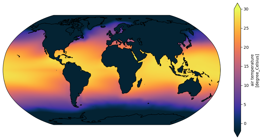
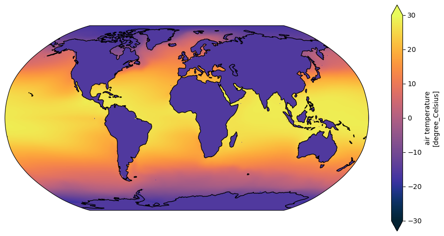
One more step is to modify the original routine to take the vertical range as an argument, so it is more generally useful:
[26]:
def map_mean_temp_in_degrees_celsius(da, vmin=-2, vmax=30):
    # Take the time mean of da and plot a global temperature field in a Robinson projection
    #
    # Input DataArray (da) should be a 3D array of latitude, longitude and time.

    da = da.pint.quantify().pint.to('C')
    da_time_mean = da.cf.mean('time')

    plt.figure(figsize=(12, 6))
    ax = plt.axes(projection=ccrs.Robinson())

    da_time_mean = da_time_mean.pint.dequantify()
    da_time_mean.cf.plot(ax=ax,
                         x='longitude', y='latitude',
                         transform=ccrs.PlateCarree(),
                         vmin=vmin, vmax=vmax, extend='both',
                         cmap=cm.cm.thermal)

    ax.coastlines()
By specifying default values for the arguments it is completely backwards compatible, we have lost no functionality, but the ice air temperature can now be plotted with a range that better suits the range of the data
[27]:
map_mean_temp_in_degrees_celsius(ice_air_temp, vmin=-30)
Conclusion
Model-specific code to take a time mean and plot the data was converted to a model agnostic function with no loss of functionality.
The same function can be used with a wide range CF-compliant data.
In some cases the input data will need to be modified if it is not sufficiently compliant, or non-conforming in some way (such as the ice data above with NaN’s in the coordinate). It is better to modify the data to be more compliant and higher quality, and use generic tools, than have multiple code versions to account for the vagaries or problems of individual datasets.
Ideally, those improvements can be incorporated into future versions of the data at source, in post-processing, or in some utility functions for transforming a class of non-conforming data.
[28]:
client.close()
[ ]: